MOOSE 系统介绍
Table of Contents
- 1. 爱达荷国家实验室 (Idaho National Laboratory)
- 2. MOOSE 简介
- 3. 创建多物理场代码
- 4. 问题陈述
- 5. 教程步骤
- 6. 第 1 步:几何与扩散
- 7. 有限元法 (Finite Element Method, FEM)
- 8. 有限元形函数
- 9. 数值实现
- 10. C++ 基础
- 11. C++ 作用域、内存和重载
- 11.1. 作用域
- 11.2. 作用域解析运算符
- 11.3. 赋值
- 11.4. 指针
- 11.5. 指针语法
- 11.6. 指针语法(续)
- 11.7. 指针功能强大但不安全
- 11.8. 引用来救场
- 11.9. 引用更安全
- 11.10. 右值引用可以更高效
- 11.11. 总结:指针和引用
- 11.12. 调用约定
- 11.13. “Swap” 示例 - 传值调用
- 11.14. Swap 示例 - 传(左值)引用
- 11.15. 动态内存分配
- 11.16. C++ 中的动态内存
- 11.17. 示例:动态内存
- 11.18. 示例:使用引用的动态内存
- 11.19. Const
- 11.20. Constexpr
- 11.21. 函数重载
- 12. C++ 类型、模板和标准模板库 (STL)
- 13. C++ 类和面向对象编程
- 14. Point 类定义 (Point.C)
- 15. 派生类:Circle.h
- 16. MOOSE C++ 标准
- 17. 代码建议
- 18. 第 2 步:压力核
- 19. MooseObject
- 20. 输入参数
- 21. Kernel 系统
- 22. 第 2 步:压力核
- 23. 动手实践:拉普拉斯-杨
- 24. 网格系统
- 25. 输出系统
- 26. 第 3 步:带材料的压力核
- 27. 材料系统
- 28. 函数系统
- 29. 第 3 步:带材料的压力核
- 30. 测试系统
- 31. 第 4 步:速度辅助变量
- 32. 辅助系统
- 33. 第 4 步:速度辅助变量
- 34. 第 5 步:热传导
- 35. Executioner 系统
- 36. 时间积分器系统
- 37. 时间步进器系统
- 38. 第 5 步:热传导
- 39. 边界条件系统
- 40. 第 5 步:热传导
- 41. 第 6 步:方程耦合
- 41.1. DarcyAdvection.h
- 41.2. DarcyAdvection.C
- 41.3. LinearInterpolation
- 41.4. LinearInterpolation
- 41.5. PackedColumn.h
- 41.6. PackedColumn.C
- 41.7. HeatConductionOutflow.h
- 41.8. HeatConductionOutflow.C
- 41.9. 第 6a 步:耦合压力和热方程
- 41.10. 变量缩放
- 41.11. 第 6a 步:运行
- 41.12. 第 6a 步:结果
- 41.13. 第 6b 步:振荡压力和温度依赖性
- 41.14. 第 6b 步:输入文件
- 41.15. 第 6b 步:运行
- 41.16. 第 6b 步:结果
- 41.17. 解耦热方程
- 42. 故障排除
- 43. 自适应系统
- 44. 第 7 步:网格自适应
- 45. 第 8 步:后处理器
- 46. UserObject 系统
- 47. 后处理器系统
- 48. 向量后处理器系统
- 49. 第 8 步:后处理器
- 50. 第 9 步:力学
- 51. 模块
- 51.1. 化学反应
- 51.2. 接触
- 51.3. 接触:摩擦熨烫问题
- 51.4. 电磁学
- 51.5. 外部 PETSc 求解器
- 51.6. 流体属性
- 51.7. 流固耦合
- 51.8. 函数展开工具
- 51.9. 地球化学
- 51.10. 热传递
- 51.11. 水平集
- 51.12. 纳维-斯托克斯
- 51.13. 纳维-斯托克斯
- 51.14. 优化
- 51.15. 相场
- 51.16. 多孔流
- 51.17. 射线追踪
- 51.18. 射线追踪:手电筒光源
- 51.19. 重构不连续伽辽金 (rDG)
- 51.20. 反应堆
- 51.21. 反应堆:微型反应堆网格划分
- 51.22. 随机工具
- 51.23. 固体力学
- 51.24. 热工水力
- 51.25. 扩展有限元法 (XFEM)
- 52. 网格系统(续)
- 53. 第 9 步:力学
- 54. 第 10 步:多尺度仿真
- 55. MultiApp 系统
- 56. 传输系统
- 57. 第 10 步:多尺度仿真
- 58. 第 11 步:自定义语法
- 59. Action 系统
- 60. 第 11 步:自定义语法
- 61. 制造解法 (MMS)
- 62. 调试
- 63. 重启和恢复系统
- 64. MOOSE 可插拔系统
- 65. Action 系统
- 66. 辅助系统
- 67. 边界条件系统
- 68. 约束系统
- 69. 控制系统
- 70. 阻尼器系统
- 71. 调试系统
- 72. DGKernel 系统
- 73. DiracKernel 系统
- 74. 分布系统
- 75. 执行器系统
- 76. Executor 系统
- 77. 函数系统
- 78. 有限体积边界条件 (FVBCs) 系统
- 79. 有限体积界面核 (FVIKs) 系统
- 80. 有限体积核系统
- 81. 几何搜索系统
- 82. 初始条件系统
- 83. 指示器系统
- 84. InterfaceKernel 系统
- 85. Kernel 系统
- 86. 线搜索系统
- 87. 标记器系统
- 88. 材料系统
- 89. 网格系统
- 90. 网格生成器系统
- 91. MultiApp 系统
- 92. 节点核系统
- 93. 输出系统
- 94. 解析器系统
- 95. 分区器系统
- 96. 位置系统
- 97. 后处理器系统
- 98. 预处理器系统
- 99. 预测器系统
- 100. 问题系统
- 101. 关系管理器系统
- 102. 报告器系统
- 103. 采样器系统
- 104. 拆分系统
- 105. 时间积分器系统
- 106. 时间步进器系统
- 107. 传输系统
- 108. UserObject 系统
- 109. 向量后处理器系统
- 110. 有限体积法 (FVM)
1. 爱达荷国家实验室 (Idaho National Laboratory)
1.0.1. INL 成立于 2005 年,是美国能源部 (Department of Energy) 领先的核能研发实验室
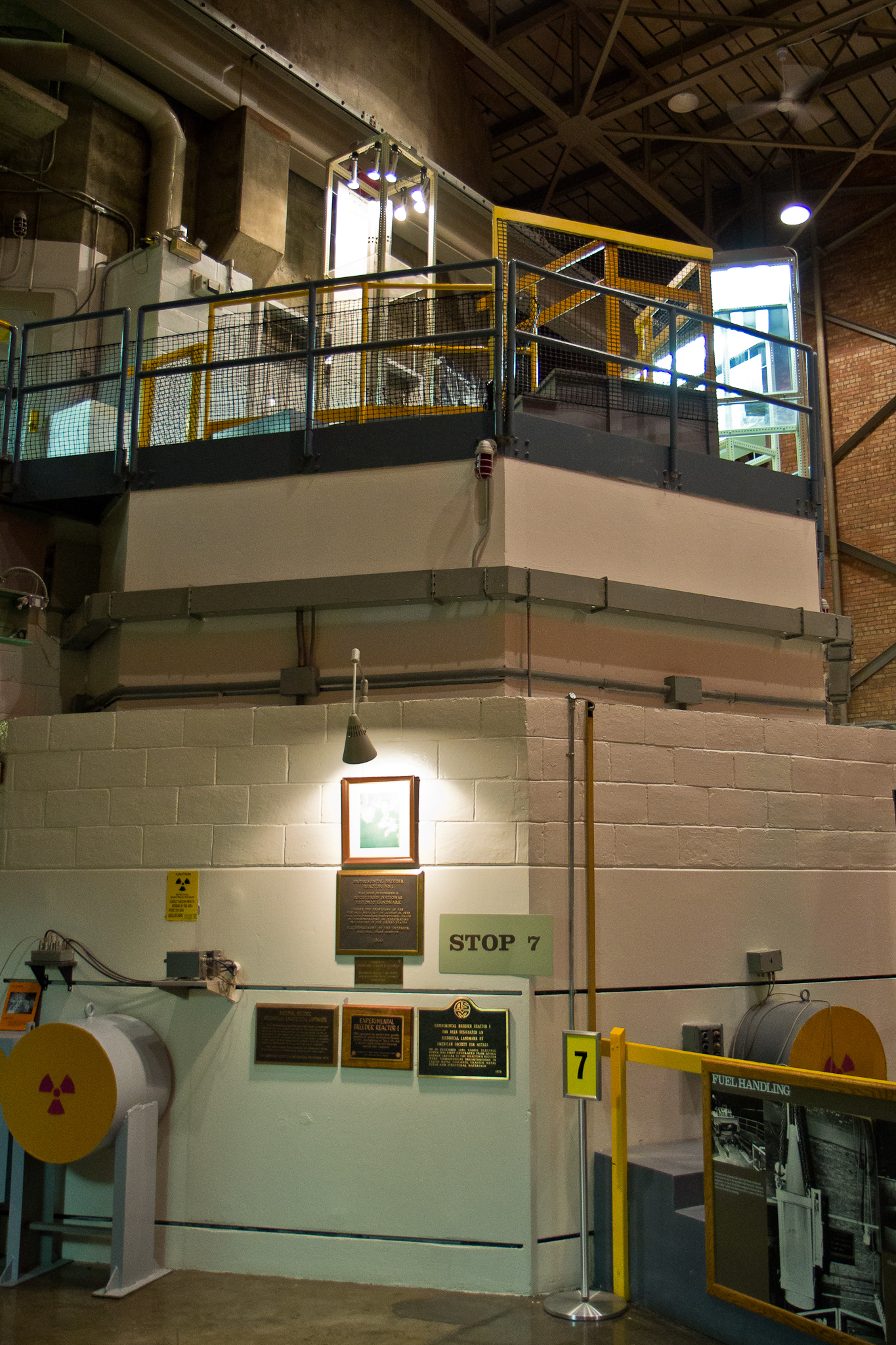
1.1. 先进测试反应堆 (Advanced Test Reactor, ATR)
世界上功率最大的测试反应堆(250 MW 热功率) 建于 1967 年 体积 1.4 立方米,含 43 千克铀,运行温度 60C
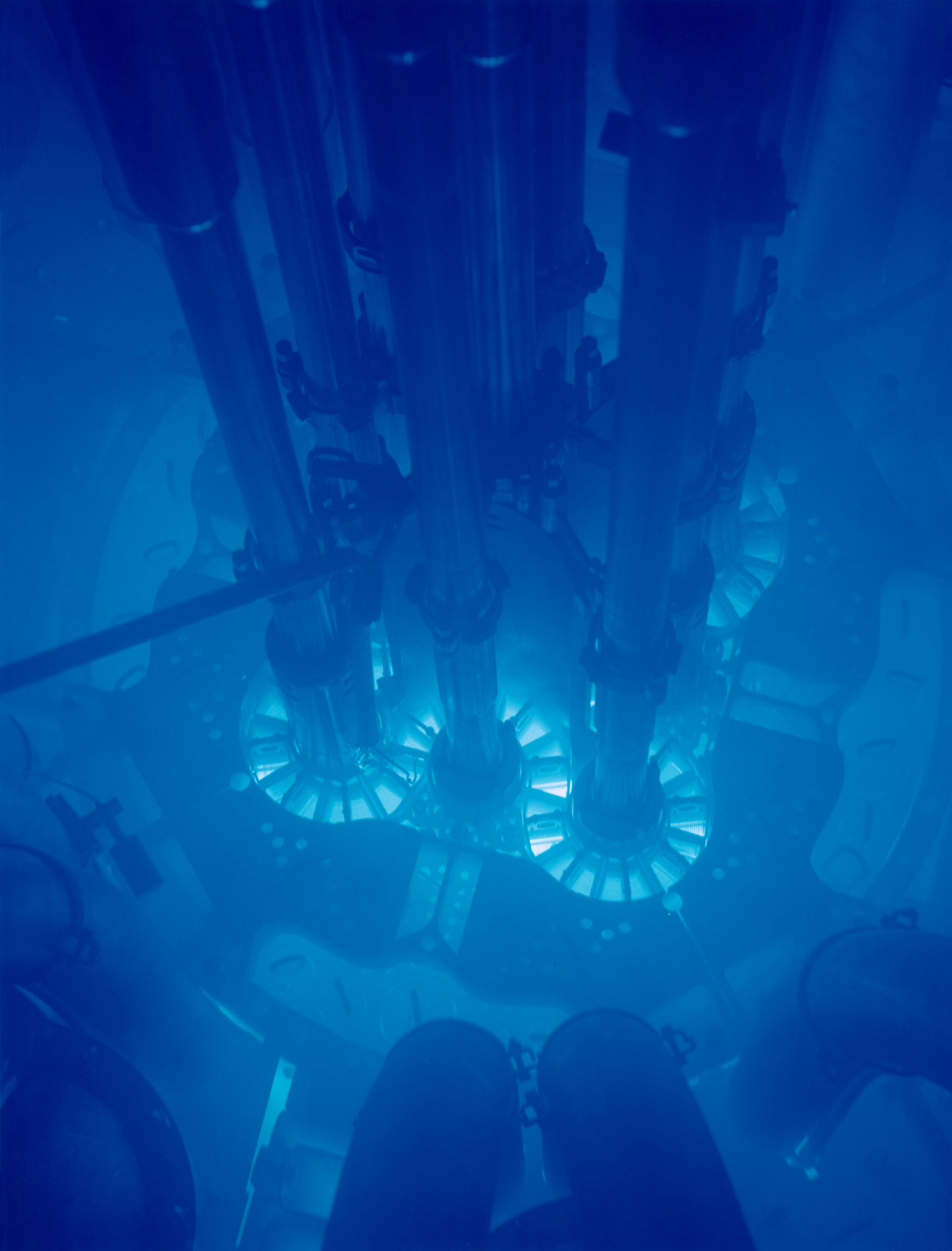
Figure 2: ATR 反应堆
1.2. 瞬态反应堆测试设施 (Transient Reactor Test Facility, TREAT)
TREAT 是一个专门设计用于评估燃料和材料在事故条件下响应的测试设施
用于严重事故测试的高强度 (20 GW)、短时 (80 ms) 中子脉冲
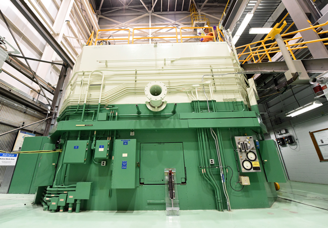
Figure 3: TREAT 设施
1.3. 国家反应堆创新中心 (National Reactor Innovation Center, NRIC)
NRIC 由两个物理试验台组成,用于建造先进核反应堆的原型
以及一个开源在线虚拟试验台,通过建模和仿真来演示先进反应堆。有关 NRIC 的更多信息,请访问 https://nric.inl.gov。
DOME (Demonstration of Microreactor Experiments) 位于历史悠久的 EBR-II 设施内,是一个能够容纳热功率低于 20MW 的运行核反应堆概念的试验台。 LOTUS (Laboratory for Operation and Testing in the U.S.) 位于历史悠久的零功率物理反应堆 (Zero Power Physics Reactor, ZPPR) 单元内, 是一个能够容纳热功率低于 500kW 的运行核反应堆概念的试验台。
2. MOOSE 简介
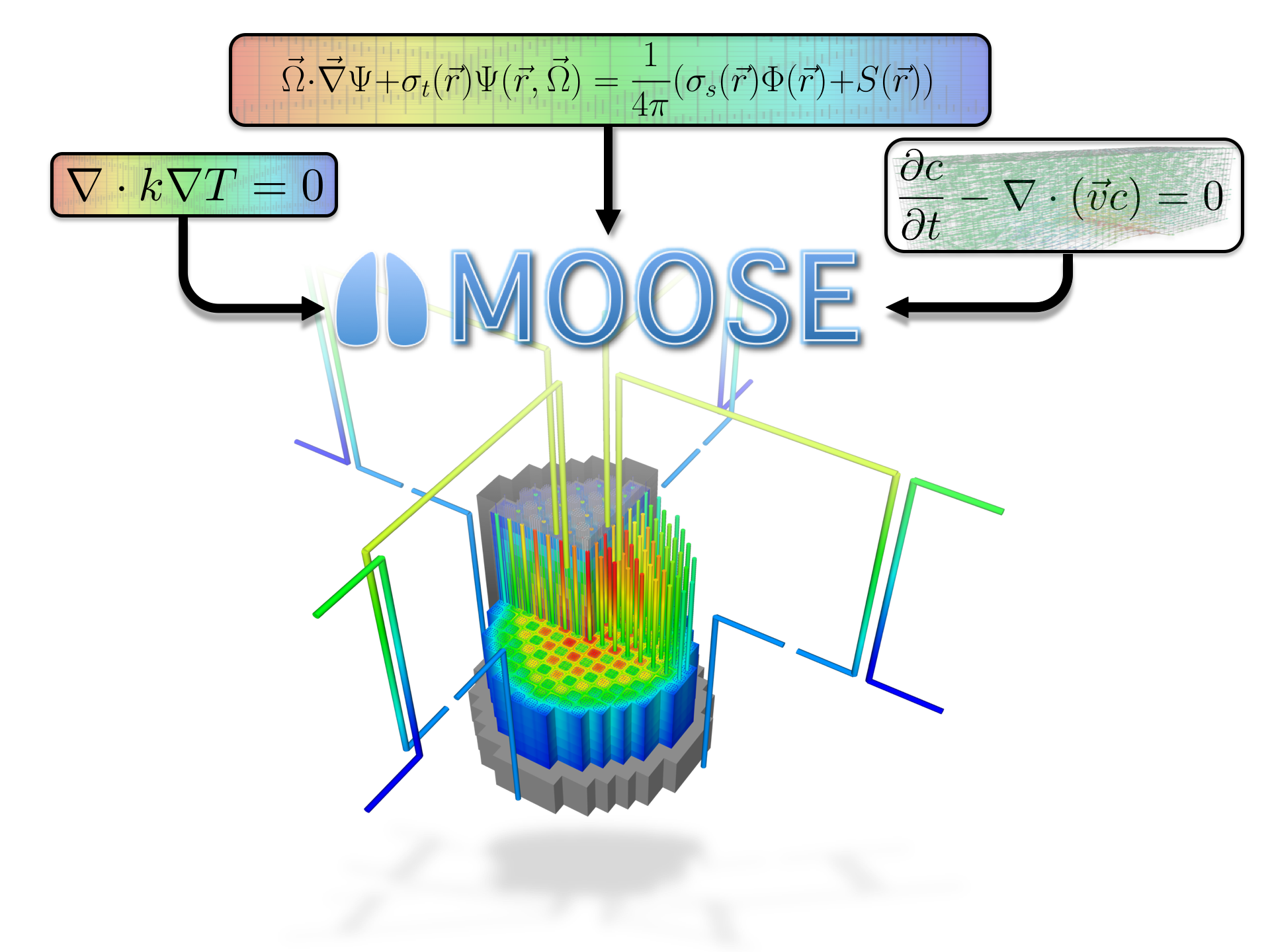
Figure 4: MOOSE 简介图
2.1. 历史与宗旨
2008 年开始开发 2014 年开源
- 旨在解决计算工程问题,并通过以下方式减少开发新应用程序所需的成本和时间:
- 易于扩展和维护
- 在少量和大量处理器上高效工作
- 提供一个面向对象的、可扩展的系统,用于创建仿真工具的各个方面
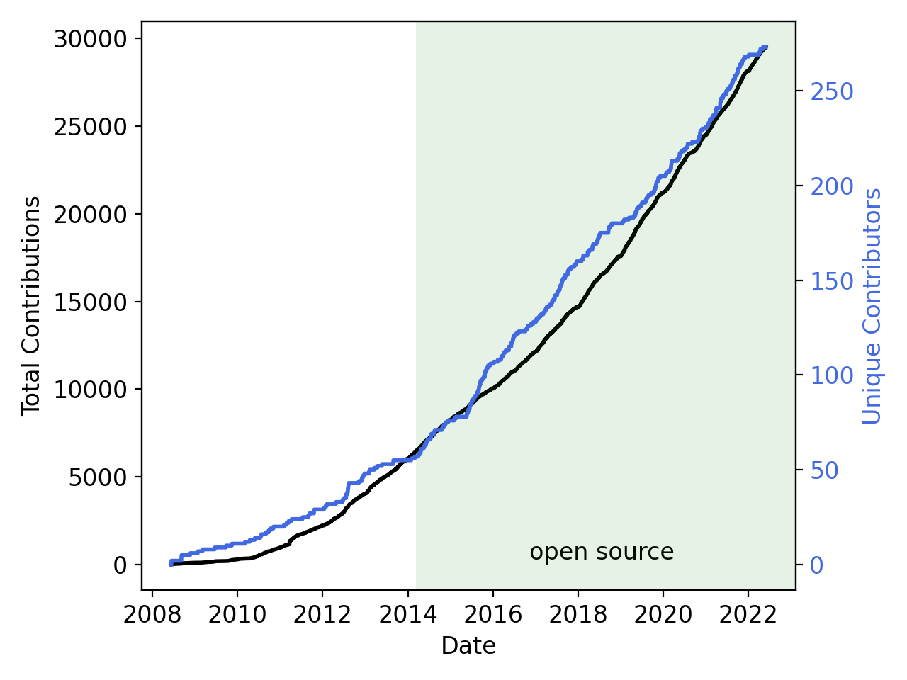
2.2. MOOSE 数据一览
- 250 位贡献者
- 56,000 次提交
- 每月 5000 名独立访客
- 每周约 40 名新的讨论参与者
- MOOSE 论文被引用 1500 次
- Elsevier Software-X 期刊中被引用次数最多的论文
- 超过 500 篇使用 MOOSE 的出版物
- 每周 3000 万次测试
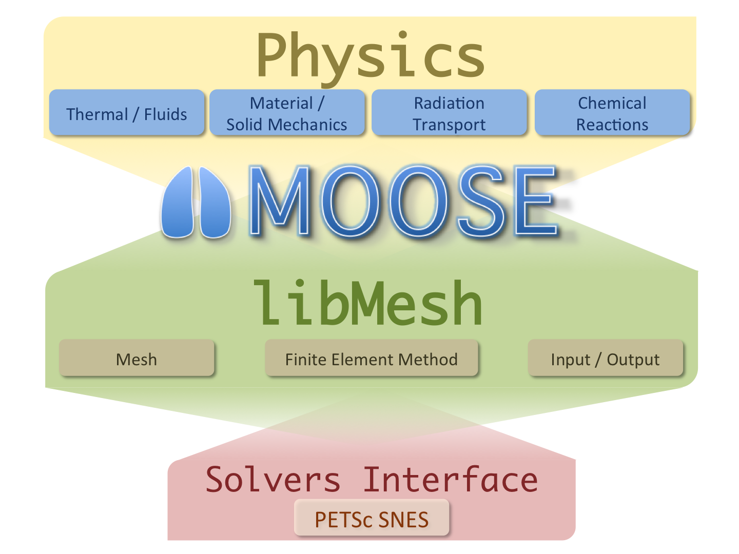
Figure 5: MOOSE 设计理念
2.3. 通用功能
- 连续和不连续伽辽金有限元法 (Continuous and Discontinuous Galerkin FEM)
- 有限体积法 (Finite Volume)
- 支持全耦合或分离系统,全隐式和显式时间积分
- 自动微分 (Automatic differentiation, AD)
- 带有限元形状的非结构化网格
- 高阶几何
- 网格自适应(加密和粗化)
- 大规模并行(MPI 和线程)
- 用户代码与维度、并行性、形函数等无关
- 操作系统:
- macOS
- Linux
- Windows (WSL)
2.4. 面向对象的、可插拔的系统
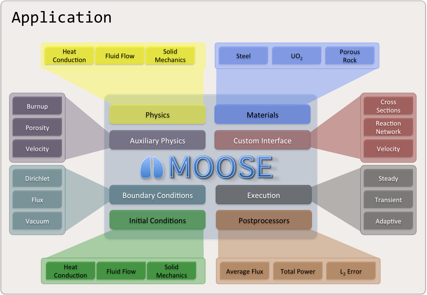
Figure 6: MOOSE 系统
2.5. 软件质量
- MOOSE 遵循核质量保证一级 (Nuclear Quality Assurance Level 1, NQA-1) 开发流程
- 所有提交都通过 GitHub Pull Requests 进行审查,并且必须通过一组应用程序回归测试,然后才能提供给我们的用户
- MOOSE 包含一个测试套件和文档系统,以支持敏捷开发,同时保持 NQA-1 流程
- 利用持续集成环境进行验证、增强和测试 (Continuous Integration Environment for Verification, Enhancement, and Testing, CIVET)
- 外部贡献由团队指导完成,我们非常欢迎!
2.6. 开发流程
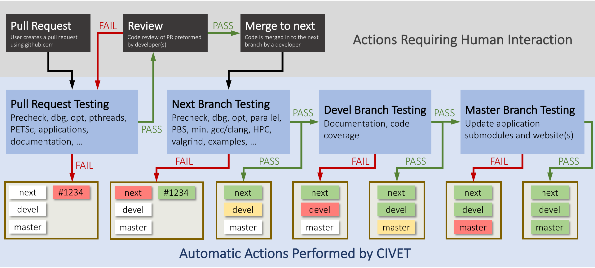
Figure 7: CIVET 流程图

2.8. 许可证
LGPL 2.1
- 不限制您对应用程序的操作
- 可以将您的应用程序作为闭源软件进行许可/销售
- 对库本身(或模块)的修改是开源的
- 新的贡献自动采用 LGPL 2.1 许可
3. 创建多物理场代码
- 多物理场很流行,但如何实现呢?
- 科学家擅长在自己的领域创建应用程序
- 那么, 跨研究小组和/或学科合作?
- 设计团队之间的迭代?
- 开发“耦合”代码?
- 有没有更好的方法?
3.1. 模块化是关键
- 数据应通过严格的接口访问,代码职责分离
- 允许代码“解耦”
- 导致更多的代码重用和更少的错误
- 对 FEM 来说具有挑战性: FEM 装配中需要形函数、自由度 (DOFs)、单元、求积点 (QPs)、材料属性、解析函数、全局积分、传输数据等等。这种复杂性使得计算科学代码脆弱且难以重用
- 需要一套一致的“系统”来执行通用操作,这些系统应通过接口进行分离
3.2. MOOSE 可插拔系统
- 系统分解责任
- 系统之间没有直接通信
- 所有东西都通过 MOOSE 接口流动
- 可以混合和匹配对象以实现仿真目标
- 输入数据可以动态更改
- 输出可以被操作(例如,对于柱坐标,乘以半径)
- 一个对象本身可以从一个应用程序中提取出来,并被另一个应用程序使用
3.3. MOOSE 可插拔系统
Actions AuxKernels Base BCs Constraints Controls Dampers DGKernels DiracKernels Distributions Executioners Functions Geomsearch ICs Indicators InterfaceKernels Kernels LineSearches Markers Materials Mesh MeshGenerators MeshModifiers Multiapps NodalKernels Outputs Parser Partitioner Positions Postprocessors Preconditioners Predictors Problems Reporters RelationshipManagers Samplers Splits TimeIntegrators TimeSteppers Transfers UserObject Utils Variables VectorPostprocessors Finite-Element Reactor Fuel Simulation
MOOSE Modules Physics Chemical Reactions Contact Electromagnetics Fluid Structure Interaction (FSI) Geochemistry Heat Transfer Level Set Navier Stokes Peridynamics Phase Field Porous Flow Solid Mechanics Thermal Hydraulics Numerics External PETSc Solver Function Expansion Tools Optimization Ray Tracing rDG Stochastic Tools XFEM Physics support Fluid Properties Solid Properties Reactor Getting started Required for upcoming hands-on Installing MOOSE Installing a text editor with input file syntax auto-complete Installing visualization software Problem Statement
3.4. 有限元反应堆燃料仿真
3.5. MOOSE 模块
3.6. MOOSE 生态系统
许多在 GitHub 上是开源的。一些可以通过 NCRC 访问
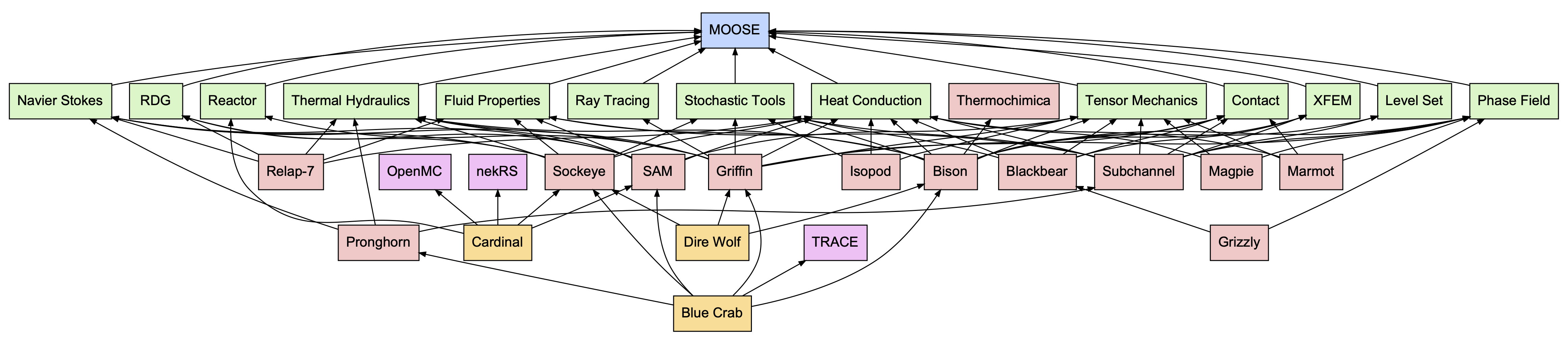
Figure 10: MOOSE 生态系统图(2022 年)
入门指南 后续动手实践所需 安装 MOOSE
安装支持输入文件语法自动补全的文本编辑器
安装可视化软件
4. 问题陈述
考虑一个包含两个不同温度压力容器的系统。这两个容器通过一根管道连接,管道中包含一个由紧密堆积的钢球组成的过滤器。预测过滤器内流体的速度和温度。管道长度为 0.304 米,直径为 0.0514 米。
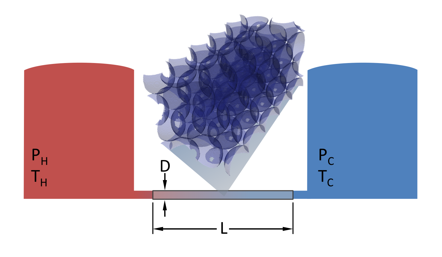
Figure 11: 问题示意图
4.1. 控制方程
质量守恒: [∇ ⋅ (ρf \mathbf{v}) = 0]
能量守恒: [(ρ cp)m \frac{\partial T}{\partial t} + (ρ cp)f \mathbf{v} ⋅ ∇ T - ∇ ⋅ (km ∇ T) = 0]
达西定律: [\mathbf{v} = -\frac{\mathbf{K}}{μf} (∇ p - ρf \mathbf{g})]
其中 (\mathbf{v}) 是流体速度,(ε) 是孔隙度,(\mathbf{K}) 是渗透率张量,(μ) 是流体粘度, p p 是压力,(ρ) 是密度, c p c p
是比热,(\mathbf{g}) 是重力矢量, T T 是温度。
假设 (ρf) 和 (μf) 是常数,并将方程 (1) 的无散条件代入方程 (3),可得到以下关于未知数 p p 和 T T 的两个方程组:
[-∇ ⋅ \left(\frac{\mathbf{K}}{μf} (∇ p - ρf \mathbf{g})\right) = 0]
[(ρ cp)m \frac{\partial T}{\partial t} + (ρ cp)f \left(-\frac{\mathbf{K}}{μf} (∇ p - ρf \mathbf{g})\right) ⋅ ∇ T = ∇ ⋅ (km ∇ T)]
参数 (ρm)、 c p m c pm
和 k m k m
是组合流体/固体介质的孔隙度相关的密度、比热容和导热系数,定义如下:
[\begin{aligned} ρm &= ε ρf + (1-ε) ρs \ (ρ cp)m &= ε (ρ cp)f + (1-ε)(ρ cp)s \ km &= ε kf + (1-ε)ks \end{aligned}]
其中 (ε) 是孔隙度, c p c p
是比热,下标 f f 和 s s 分别指流体和固体。
4.2. 材料属性
(ε = 0.39) (μf = 7.98 × 10⁻⁴ \text{ Pa} ⋅ \text{s}) ( ρ c p ) f = 4.192 × 10 6 J / ( m 3 ⋅ K ) (ρc p ) f =4.192×10 6 J/(m 3 ⋅K) k f = 0.6 W / ( m ⋅ K ) k f =0.6 W/(m⋅K) (ρf = 995.6 \text{ kg} / \text{m}3) (\mathbf{g} = [0, -9.81, 0] \text{ m}/\text{s}2) (\mathbf{K}) 是一个对角张量,其中对角线元素为 K K K 1 mm spheres = 0.8451 × 10 − 9 m 2 K 1mm spheres =0.8451×10 −9 m 2
K 3 mm spheres = 8.968 × 10 − 9 m 2 K 3mm spheres =8.968×10 −9 m 2
( ρ c p ) s = 3.728 × 10 6 J / ( m 3 ⋅ K ) (ρc p ) s =3.728×10 6 J/(m 3 ⋅K) k s = 16.3 W / ( m ⋅ K ) k s =16.3 W/(m⋅K) (ρs = 8000 \text{ kg} / \text{m}3) T i n l e t = 350 K T inlet =350 K T o u t l e t = 300 K T outlet =300 K
5. 教程步骤
5.1. 第 1 步:几何与扩散
第一步是解决一个简单的“扩散”问题,这不需要任何代码。此步骤将介绍 MOOSE 的基本系统。
[-∇ ⋅ (D ∇ u) = 0]
5.2. 第 2 步:压力核
为了实现达西压力方程,需要一个 Kernel 对象来表示:
[-∇ ⋅ (\frac{\mathbf{K}}{μ} ∇ p)]
5.3. 第 3 步:带材料的压力核
可以使用 Material 系统来提供值,而不是将常量参数传递给压力扩散 Kernel 对象。这使得属性可以随空间和时间变化,并与仿真中的变量耦合。
5.4. 第 4 步:速度辅助变量
速度是根据达西定律从压力计算出来的:
可以使用 Auxiliary 系统计算此速度。
[\mathbf{v} = -\frac{\mathbf{K}}{μf} ∇ p]
5.5. 第 5 步:热传导
使用“heat conduction”模块求解瞬态热方程。
[ρ cp \frac{\partial T}{\partial t} - ∇ ⋅ (k ∇ T) = 0]
5.6. 第 6 步:方程耦合
通过向热方程添加平流项,在耦合方程组中求解压力和温度。
[ρf cpf \mathbf{v} ⋅ ∇ T]
5.7. 第 7 步:网格自适应
在瞬态仿真中,“行波”轮廓穿过多孔介质。我们可以动态地使网格适应解,而不是使用均匀网格来解析波轮廓。
5.8. 第 8 步:后处理器
Postprocessor 和 VectorPostprocessor 对象可用于计算仿真的聚合值,例如边界上的平均温度或解域内沿某条线的温度。
5.9. 第 9 步:力学
可以使用“solid mechanics”模块将多孔介质的热膨胀添加到耦合方程组中,而无需添加额外代码。
5.10. 第 10 步:多尺度仿真
MOOSE 能够将多个应用程序一起运行,并在各个应用程序之间传输数据。
此问题将用另一个应用程序计算的值替换 Material 计算的导热系数,该应用程序运行基于相的微观结构仿真。
5.11. 第 11 步:自定义语法
MOOSE 包含一个系统,可为常见任务创建自定义输入语法,在此步骤中,为最终用户简化了两个方程和速度辅助计算的语法。
6. 第 1 步:几何与扩散
首先,考虑域上的稳态扩散方程:求解 u u ,使得
[-∇ ⋅ ∇ u = 0]
其中左边界 u = 4000 u=4000 ,右边界 u = 0 u=0 ,其余边界 (\frac{\partial u}{\partial n}=0)。
该方程的弱形式,以内积表示法,由下式给出:
[(∇ ψi, ∇ uh) = 0]
其中 (ψi) 是测试函数, u h u h
是有限元解。
6.1. 输入文件
输入文件用于在 MOOSE 中表示问题。它遵循非常标准化的语法。
MOOSE 使用“分层输入文本”(hierarchical input text, hit) 格式。
[Kernels]
[diffusion]
type = ADDiffusion # 使用自动微分的拉普拉斯算子
variable = pressure # 对上面的 "pressure" 变量进行操作
[]
[]
一个基本的 MOOSE 输入文件需要六个部分,稍后将更详细地介绍每个部分。
[Mesh]: 定义域的几何形状 [Variables]: 定义问题的未知数 [Kernels]: 定义要解的方程 [BCs]: 定义问题的边界条件 [Executioner]: 定义问题的求解方式 [Outputs]: 定义解的返回方式
6.2. 第 1 步:输入文件
[Mesh]
[gmg]
type = GeneratedMeshGenerator # 可以生成简单的线、矩形和长方体
dim = 2 # 网格维度
nx = 100 # x 方向的单元数
ny = 10 # y 方向的单元数
xmax = 0.304 # 测试室长度
ymax = 0.0257 # 测试室半径
[]
coord_type = RZ # 轴对称 RZ
rz_coord_axis = X # 对称轴
[]

[Variables/pressure]

默认添加一个线性拉格朗日变量
[]

[Kernels/diffusion]
type = ADDiffusion # 使用自动微分的拉普拉斯算子
variable = pressure # 对上面的 "pressure" 变量进行操作
[]

[BCs]
[inlet]
type = DirichletBC # 简单的 u=value 边界条件
variable = pressure # 要设置的变量
boundary = left # 网格中的一个边集名称
value = 4000 # (Pa) 来自论文图 2。1mm 球体的第一个数据点。
[]
[outlet]
type = DirichletBC
variable = pressure
boundary = right
value = 0 # (Pa) 根据图 2 给出 1mm 球体的正确压降
[]
[]

[Problem]
type = FEProblem # 这是 MOOSE 中“正常”类型的有限元问题
[]

[Executioner]
type = Steady # 稳态问题
solve_type = NEWTON # 执行牛顿求解,使用 AD 计算雅可比项
petsc_options_iname = '-pc_type -pc_hypre_type' # PETSc 选项对,值在下面
petsc_options_value = 'hypre boomeramg'
[]

[Outputs]
exodus = true # 输出 Exodus 格式
[]
6.3. 第 1 步:运行
通过编译应用程序或 MOOSE 模块生成可执行文件。它可用于运行输入文件。
cd ~/projects/moose/tutorials/darcy_thermo_mech/step01_diffusion
make -j 12 # 使用您系统的处理器数量
cd problems
../darcy_thermo_mech-opt -i step1.i
6.4. 第 1 步:结果

Figure 12: 步骤 1 的结果图
7. 有限元法 (Finite Element Method, FEM)
7.1. 函数逼近
为了引入 FEM 的概念,考虑一个多项式回归练习。我们可以寻找一个多项式函数来解决以下问题:
[y(x) ≈ f(x)]
让我们将多项式写成以下形式:
[y(x) = ∑j=0n cj φj(x)]
其中 c j c j
是标量系数(展开系数),单项式 (φj(x)) 是“基函数”。因此,问题是找到 c j c j
使得 y ( x ) y(x) 最接近给定的点或给定的函数。
离散示例:给定采样位置及相关值,我们希望我们的多项式函数尽可能接近输入数据。 连续示例:给定一个复杂函数,我们希望我们的多项式函数尽可能接近输入函数。
7.2. 多项式示例(离散)
y 0 = c 0
c 1 x 0
c 2 x 0 2
c 3 x 0 3 y 1 = c 0
c 1 x 1
c 2 x 1 2
c 3 x 1 3 y 2 = c 0
c 1 x 2
c 2 x 2 2
c 3 x 2 3 y 3 = c 0
c 1 x 3
c 2 x 3 2
c 3 x 3 3
y 0
y 1
y 2
y 3
=c 0 +c 1 x 0 +c 2 x 0 2 +c 3 x 0 3
=c 0 +c 1 x 1 +c 2 x 1 2 +c 3 x 1 3
=c 0 +c 1 x 2 +c 2 x 2 2 +c 3 x 2 3
=c 0 +c 1 x 3 +c 2 x 3 2 +c 3 x 3 3
( y 0 y 1 y 2 y 3
) = ( 1 x 0 x 0 2 x 0 3 1 x 1 x 1 2 x 1 3 1 x 2 x 2 2 x 2 3 1 x 3 x 3 2 x 3 3
) ( c 0 c 1 c 2 c 3
)
y 0
y 1
y 2
y 3
=
1 1 1 1
x 0
x 1
x 2
x 3
x 0 2
x 1 2
x 2 2
x 3 2
x 0 3
x 1 3
x 2 3
x 3 3
c 0
c 1
c 2
c 3
[\mathbf{y} = \mathbf{V} \mathbf{c}]
[\mathbf{c} = \mathbf{V}-1 \mathbf{y}]
( y 0 y 1 y 2 y 3
) = ( 1.0 0.2 2.0 1.0
) ( x 0 x 1 x 2 x 3
) = ( − 1.0 − 0.5 0.5 1.0
)
y 0
y 1
y 2
y 3
=
1.0 0.2 2.0 1.0
x 0
x 1
x 2
x 3
=
−1.0 −0.5 0.5 1.0
( c 0 c 1 c 2 c 3
) = ( 0.925 − 3.933 1.800 2.267
)
c 0
c 1
c 2
c 3
=
0.925 −3.933 1.800 2.267
[y(x) = c0 + c1 x + c2 x2 + c3 x3]
[y(0.1) = 0.925 - 3.933(0.1) + 1.8(0.1)2 + 2.267(0.1)3 = 0.552]
这些系数定义了解函数:
[y(x) = 0.925 - 3.933 x + 1.8 x2 + 2.267 x3]
7.3. 多项式示例(连续)
[∫-11 (f(x) - yh(x))2 dx = ∫-11 \left(f(x) - ∑j=0n cj φj(x)\right)2 dx]
[\frac{\partial}{\partial c_i} ∫-11 \left(f(x) - ∑j=0n cj φj(x)\right)2 dx = 0]
[∫-11 2 \left(f(x) - ∑j=0n cj φj(x)\right) (-φi(x)) dx = 0]
[∫-11 f(x)φi(x) dx = ∑j=0n cj ∫-11 φj(x)φi(x) dx]
[\mathbf{F}i = ∑{j=0}n cj \mathbf{M}ij]
[\mathbf{M} \mathbf{c} = \mathbf{F}]
[\mathbf{c} = \mathbf{M}-1 \mathbf{F}]
对于 f ( x ) = sin ( 2 π x ) f(x)=sin(2πx) 和 (φj(x) = xj),我们得到 c = [ − 0.0 , − 0.73 , 0.0 , 3.48 ] c=[−0.0,−0.73,0.0,3.48] 。
这些系数定义了解函数:
[y(x) = -0.73x + 3.48x3]
系数是无意义的,它们只是用来定义函数的数字。
解 不是 系数,而是当它们乘以各自的基函数并相加时创建的 函数。
函数 y h ( x ) y h (x) 在域中的任何地方都有定义。
y h ( x ) y h (x) 可以在点 x = 0.1 x=0.1 处求值,例如,通过计算:
[yh(0.1) = ∑j=03 cj φj(0.1)]
其中 c j c j
对应于解向量中的系数,(φj) 是各自的函数。
7.4. FEM 可用于求解线性和非线性 PDE
FEM 是一种数值逼近偏微分方程 (PDE) 解的方法。FEM 广泛适用于各种 PDE 和域。
示例 PDE:您以前见过它们吗?它们是线性的/非线性的?耦合的?
[-∇ ⋅ ∇ u = f]
[\frac{\partial u}{\partial t} - ∇ ⋅ (D∇ u) + \mathbf{v} ⋅ ∇ u = f]
[-∇ ⋅ σ = f, \quad σ = C:(ε - ε0), \quad ε = \frac{1}{2}(∇ \mathbf{u} + (∇ \mathbf{u})T)]
7.5. FEM 是离散化这些方程的通用方法
FEM 找到一个由“形函数”乘以系数并相加组成的解函数,就像多项式回归一样,只是函数通常不那么简单(尽管它们可以是)。
伽辽金有限元法与有限差分法和有限体积法不同,因为它找到一个分段连续函数,该函数是控制 PDE 的近似解。
FEM 提供一个近似解。真实解只能被形函数基底所能表示的程度来表示!
FEM 有丰富的数学理论支持,有关于精度、稳定性、收敛性和解唯一性的证明。
7.6. 弱形式
使用 FEM 求解 PDE 首先要形成一个“加权残差”或“变分陈述”或“弱形式”,此过程在此处称为生成弱形式。
弱形式在数学上和数值上都提供了灵活性,MOOSE 需要它来解决问题。
生成弱形式通常涉及以下步骤:
写出方程的强形式 重新排列以在右侧得到零 乘以测试函数 (ψi) 在域 (Ω) 上积分 对包含最高阶导数的项进行分部积分
7.7. 回顾
多项式拟合:
形成多项式函数的系数必须满足的方程以进行拟合 求解线性系统 通过评估由其系数定义的多项式来重建拟合 有限元法:
在每个单元上形成方程以最小化方程的残差 求解线性系统 重建函数 重新评估方程并迭代(对于非线性方程)
7.8. 分部积分和散度定理
假设 (φ) 是一个标量函数,(\mathbf{F}) 是一个向量函数,并且两者都是连续可微的函数,则乘积法则表明:
[∇ ⋅ (φ \mathbf{F}) = (∇ φ) ⋅ \mathbf{F} + φ (∇ ⋅ \mathbf{F})]
该函数可以在体积 (Ω) 上积分并重新排列为:
[∫Ω φ (∇ ⋅ \mathbf{F}) dV = ∫Ω ∇ ⋅ (φ \mathbf{F}) dV - ∫Ω (∇ φ) ⋅ \mathbf{F} dV]
散度定理将体积积分转换为表面 (∂Ω) 上的面积分:
[∫Ω ∇ ⋅ \mathbf{G} dV = \oint∂Ω \mathbf{G} ⋅ \mathbf{n} dS]
其中 (\mathbf{n}) 是表面 (∂Ω) 的外法线向量。结合方程 (7) 和方程 (8) 可得:
[∫Ω φ (∇ ⋅ \mathbf{F}) dV = \oint∂Ω φ \mathbf{F} ⋅ \mathbf{n} dS - ∫Ω (∇ φ) ⋅ \mathbf{F} dV]
7.9. 示例:平流-扩散
(1) 写出方程的强形式:
[-∇ ⋅ (D ∇ u) + ∇ ⋅ (\mathbf{v}u) = f]
(2) 重新排列以在右侧得到零:
[-∇ ⋅ (D ∇ u) + ∇ ⋅ (\mathbf{v}u) - f = 0]
(3) 乘以测试函数 (ψi):
[ψi(-∇ ⋅ (D ∇ u) + ∇ ⋅ (\mathbf{v}u) - f) = 0]
(4) 在域 (Ω) 上积分:
[∫Ω ψi(-∇ ⋅ (D ∇ u) + ∇ ⋅ (\mathbf{v}u) - f) dV = 0]
(5) 使用方程 (9) 对 PDE 的最左边项进行分部积分并应用散度定理:
[∫Ω (∇ψi, D∇ u) dV - ∫∂Ω ψi D ∇ u ⋅ \mathbf{n} dS - ∫Ω (∇ψi, \mathbf{v}u) dV + ∫∂Ω ψi \mathbf{v}u ⋅ \mathbf{n} dS - ∫Ω (ψi, f) dV = 0]
以内积表示法书写。方程的每一项都将继承自现有的 MOOSE 类型,如下所示。
[(∇ ψi, D ∇ u) - ⟨ ψi, D ∇ u ⋅ \mathbf{n} ⟩∂Ω - (∇ ψi, \mathbf{v}u) + ⟨ ψi, \mathbf{v}u ⋅ \mathbf{n} ⟩∂Ω - (ψi, f) = 0]
7.10. 相应的 MOOSE 输入文件块
[Kernels]
[diff]
type = Diffusion
variable = u
[]
[]
[BCs]
[right]
type = NeumannBC
variable = u
boundary = 1
value = 1
[]
[]
[Kernels]
[adv_u]
implicit = false
type = ConservativeAdvection
variable = u
velocity = '1 0 0'
[]
[]
[Kernels]
[ffn]
type = BodyForce
variable = u
function = f_fn
[]
[]
[\underbrace{(\nabla \psi_i, D \nabla u)}{\text{Diffusion Kernel}} - \underbrace{⟨ ψi, D ∇ u ⋅ \mathbf{n} ⟩{∂Ω}}{\text{Neumann BC}} - \underbrace{(∇ ψi, \mathbf{v}u)}{\text{Advection Kernel}} + … - \underbrace{(\psi_i, f)}\text{BodyForce Kernel}]
8. 有限元形函数
8.1. 基函数

Figure 13: FEM 帽函数
Figure 14: FEM 基函数
8.2. 形函数
u u 的离散化展开式采用以下形式:
[uh = ∑j=1Ndof uj φj(\mathbf{x})]
其中 (φj) 是“基函数”,它们构成了“试探函数” u h u h
的基础。 N d o f N dof
是离散化域的函数总数。
u h u h
的梯度可以类似地展开:
[∇ uh = ∑j=1Ndof uj ∇ φj(\mathbf{x})]
在伽辽金有限元法中,试探函数和测试函数使用相同的基函数:
[ψi = φi]
将这些展开式代入示例弱形式(方程 (10))中,得到:
[∑j=1Ndof uj \left[ (∇ φi, D ∇ φj) - (∇ φi, \mathbf{v}φj) \right] - ⟨ φi, D ∇ uh ⋅ \mathbf{n} ⟩∂Ω - (φi, f) = 0 \quad ∀ i]
上面方程的左侧被称为“残差向量” (\mathbf{R}) 的第 i i 个分量。
形函数是乘以系数并相加形成解的函数。
单个形函数是全局基函数在单个单元上的限制。
它们类似于多项式拟合中的 (φj(x)) 函数(实际上,您可以将那些用作形函数)。
典型的形函数族:Lagrange, Hermite, Hierarchic, Monomial, Clough-Toucher
Lagrange 形函数是最常见的,它们在节点处是插值性的,即系数对应于函数在节点处的值。
8.3. 示例一维形函数

Figure 15: 线性 Lagrange

Figure 16: 二次 Lagrange
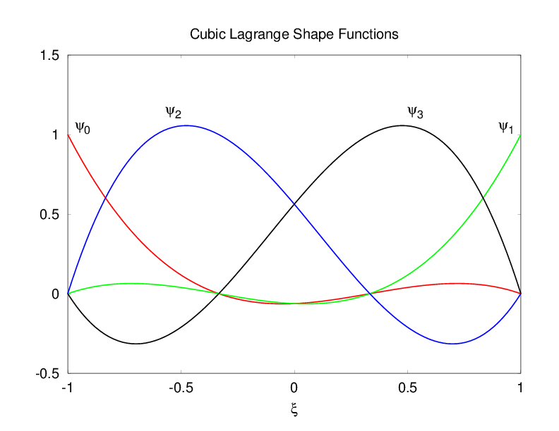
Figure 17: 三次 Lagrange
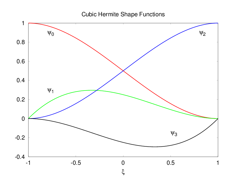
Figure 18: 三次 Hermite
8.4. 二维 Lagrange 形函数
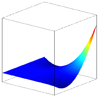
Figure 19: (φ0)
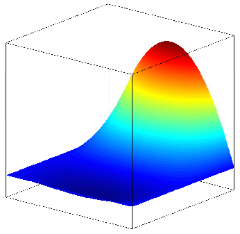
Figure 20: (φ4)
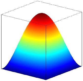
Figure 21: (φ8)
(φ0 = \frac{1}{4} ξ η (ξ - 1) (η - 1)) (φ4 = \frac{1}{2} (1 - ξ2) η (η - 1)) (φ8 = (1 - ξ2) (1 - η2)) (∑j φj = 1)
8.5. 在 MOOSE 输入文件中设置形函数
可以在 Variables 块中为每个变量设置形函数:
[Variables]
[u]
order = FIRST
family = LAGRANGE
block = 0
[]
[v]
order = FIRST
family = LAGRANGE
block = 1
[]
[]
9. 数值实现
9.1. 数值积分
弱形式中唯一剩下的非离散化部分是积分。首先,将域积分分解为单元积分之和:
[∫Ω … dV = ∑e ∫Ωe … dV]
通过变量变换,单元积分被映射到“参考”单元上的积分。
[∫Ωe … dV = ∫\hat{\Omega} … |J| d\hat{V}]
其中 ∣ J ∣ ∣J∣ 是从物理单元到参考单元的映射的雅可比行列式。
9.2. 参考单元 (Quad9)

Figure 22: Quad9 参考单元
9.2.1. 求积
求积,通常是“高斯求积”,用于数值逼近参考单元积分。
[∫\hat{\Omega} \hat{g} d\hat{V} ≈ ∑q=1Nqp \hat{g}(\hat{\mathbf{x}}q) wq]
其中 w q w q
是求积点 (\hat{\mathbf{x}}q) 处的权函数。
在某些常见情况下,求积逼近是精确的。例如,在一维中,高斯求积可以用 n q p n qp
个求积点精确地积分 2 n q p − 1 2n qp −1 阶多项式。
将求积应用于方程 (12),我们可以简单地计算:
[∫Ωe g(\mathbf{x}) dV = ∫\hat{\Omega} \hat{g}(\hat{\mathbf{x}})|J| d\hat{V} ≈ ∑q=1Nqp \hat{g}(\hat{\mathbf{x}}q) |J(\hat{\mathbf{x}}q)| wq]
其中 (\mathbf{x}q) 是第 q q 个求积点的空间位置, w q w q
是其相关的权重。
MOOSE 自动处理乘以雅可比行列式 ( ∣ J ∣ ∣J∣ ) 和权重 ( w q w q
),因此您的 Kernel 对象只负责计算被积函数的 (\hat{g}) 部分。
在求积点处对 u h u h
和 (∇ uh) 进行采样得到:
[uh(\mathbf{x}q) = ∑{j=1}Ndof uj φj(\mathbf{x}q) \quad ∇ uh(\mathbf{x}q) = ∑{j=1}N{dof} uj ∇ φj(\mathbf{x}q)]
因此,方程 (11) 的弱形式变为:
[Ri = ∑e \left[ ∑q=1Nqp \left[ D(\mathbf{x}q) ∑{j=1}Ndof uj ∇φj(\mathbf{x}q) ⋅ ∇φi(\mathbf{x}q) - \mathbf{v}(\mathbf{x}q) ∑{j=1}N{dof} uj φj(\mathbf{x}q) ⋅ ∇φi(\mathbf{x}q) - f(\mathbf{x}q) φi(\mathbf{x}q) \right] |J(\mathbf{x}q)| wq - ∑{fq=1}N{fq} … \right]]
第二个求和是在边界小平面 f f 上。MOOSE Kernel 或 BoundaryCondition 对象分别提供方括号中的每一项(在 (\mathbf{x}q) 或 (\mathbf{x}{fq}) 处求值)。
9.3. 中间总结
有一个网格,包含单元和函数,多项式,由其系数定义 我们将这些函数代入 PDE,然后得到一个弱形式 我们使用求积法评估弱形式中的积分,从而形成一组方程 现在让我们求解这些方程以获得系数
9.4. 牛顿法
牛顿法是一种具有良好收敛性的“求根”方法,以“更新形式”表示,用于求解标量方程的根,定义为: x k
1 = x k − f ( x k ) f ′ ( x k ) x k+1 =x k − f ′ (x k ) f(x k )
,(δ x = xk+1 - xk) 由下式给出:
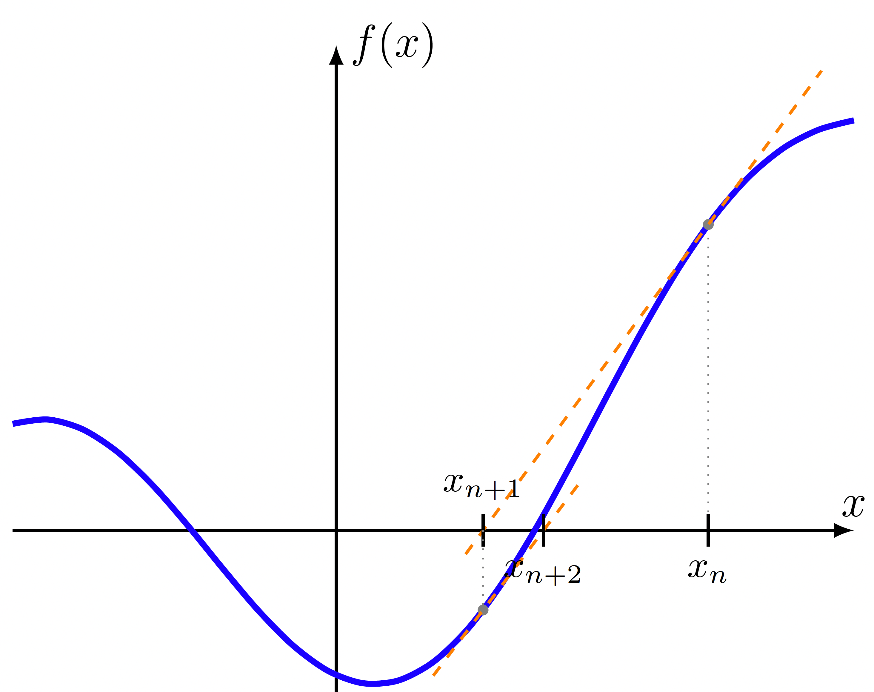
Figure 23: 牛顿法
[f'(xk)δ x = -f(xk)]
9.5. MOOSE 中的牛顿法
由方程 (13) 定义的残差 (\mathbf{R}(\mathbf{u})) 是一个非线性方程组,
[\mathbf{R}(\mathbf{u}) = \mathbf{0}]
用于求解系数 (\mathbf{u})。
对于这个非线性方程组,牛顿法定义为:
[\mathbf{J}(\mathbf{u}k) δ \mathbf{u} = -\mathbf{R}(\mathbf{u}k), \quad \mathbf{u}k+1 = \mathbf{u}k + δ \mathbf{u}]
其中 (\mathbf{J}) 是在当前迭代 (\mathbf{u}k) 处求值的雅可比矩阵:
[Jij = \frac{\partial R_i}{\partial u_j}]
9.6. MOOSE 求解类型
求解类型在输入文件的 [Executioner] 块中指定:
可用选项包括:
PJFNK: Preconditioned Jacobian Free Newton Krylov (默认) JFNK: Jacobian Free Newton Krylov NEWTON: 使用精确雅可比进行预处理求解 FD: PETSc 使用有限差分法计算项 (调试)
[Executioner]
solve_type = PJFNK
9.7. JFNK
使用基于 Krylov 子空间的线性求解器
雅可比的作用通过以下方式逼近:
[\mathbf{J}\mathbf{v} ≈ \frac{\mathbf{R}(\mathbf{u} + ε\mathbf{v}) - \mathbf{R}(\mathbf{u})}{ε}]
Kernel 方法 computeQpResidual 被调用以在非线性步骤(方程 (14))中计算 (\mathbf{R}(\mathbf{u}k))。
在 JFNK 的每个线性步骤中,都会调用 computeQpResidual 方法来逼近雅可比对 Krylov 向量的作用。
9.8. PJFNK
预处理雅可比的作用通过以下方式逼近:
[\mathbf{P}-1\mathbf{J}\mathbf{v} ≈ \mathbf{P}-1\frac{\mathbf{R}(\mathbf{u} + ε\mathbf{v}) - \mathbf{R}(\mathbf{u})}{ε}]
Kernel 方法 computeQpResidual 被调用以在非线性步骤(方程 (14))中计算 (\mathbf{R}(\mathbf{u}k))。
在 PJFNK 的每个线性步骤中,都会调用 computeQpResidual 方法来逼近雅可比对 Krylov 向量的作用。computeQpJacobian 和 computeQpOffDiagJacobian 方法用于计算预处理矩阵的值。
9.9. NEWTON
Kernel 方法 computeQpResidual 被调用以在非线性步骤(方程 (14))中计算 (\mathbf{R}(\mathbf{u}k))。
computeQpJacobian 和 computeQpOffDiagJacobian 方法用于计算预处理矩阵。假设预处理矩阵就是雅可比矩阵,因此残差和雅可比计算在线性迭代期间可以保持不变。
9.10. 预处理
使用 PETSC 选项选择预处理器,可以在 executioner 中或在 [Preconditioning] 块中:
一些示例:
对于并行预处理器,子块(进程上)预处理器可以用 PETSc 选项 -subpctype 控制。例如,对于并行块 Jacobi 预处理器 (-pctype bjacobi),子块预处理器可以设置为 ILU 或 LU 等,使用 -subpctype ilu,-subpctype lu 等。
LU : 形成实际的雅可比逆,适用于中小型问题,但扩展性不佳 Hypre BoomerAMG : 代数多重网格,适用于扩散问题 Jacobi : 使用雅可比的对角线、行和或行最大值进行预处理
[Executioner]
type = Steady
petsc_options_iname = '-pc_type -pc_hypre_type'
petsc_options_value = 'hypre boomeramg'
9.11. 总结
有限元法是一种数值逼近 PDE 解的方法。
就像多项式拟合一样,FEM 找到基函数的系数。
解是系数和基函数的组合,解可以在域中的任何地方采样。
积分使用求积法进行数值计算。
牛顿法提供了一种求解非线性方程组的机制。
预处理的无雅可比牛顿-克雷洛夫 (PJFNK) 方法使我们能够避免显式形成雅可比矩阵,同时仍然计算其作用。
9.12. 自动雅可比计算
MOOSE 使用来自 MetaPhysicL 包的前向模式自动微分。
未来,我们的想法是让应用程序开发人员能够在不编写任何雅可比语句的情况下开发整个应用程序。这有可能减少应用程序开发时间。
在计算性能方面,目前 AD 雅可比的计算速度比手动编码的雅可比慢,但它们并行化得非常好,并且可以从使用 NEWTON 求解中受益,这通常会减少整体求解时间。
依赖于两种技术:
链式法则 运算符重载 [\frac{\partial f(g(x))}{\partial x} = \frac{\partial f}{\partial g} \frac{\partial g}{\partial x}]
需要注意的一点是,导数是关于自由度的,但残差是在求积点计算的!因此,即使对于简单的 u ( x q ) u(x q ) (变量 u u 在求积点的值),也常常有多个非零系数。
[\frac{∂ u(\mathbf{x}q)}{∂ uj} = φj(\mathbf{x}q)]
9.13. 手动雅可比计算
本教程的其余部分将重点介绍使用自动微分 (AD) 计算雅可比项,但也可以手动计算它们。
建议所有新的 Kernel 对象都使用 AD。
9.13.1. FEM 导数恒等式
在计算雅可比项时,以下关系式很有用。
[\frac{\partial u_h}{\partial u_j} = φj]
[\frac{\partial \nabla u_h}{\partial u_j} = ∇φj]
9.13.2. 简单方程的牛顿法
再次考虑具有非线性 D ( u ) D(u) 、(\mathbf{v}(u)) 和 f ( u ) f(u) 的平流-扩散方程:
[-∇ ⋅ (D(u) ∇ u) + \mathbf{v}(u) ⋅ ∇ u = f(u)]
因此,残差向量的第 i i 个分量是:
[Ri = (∇ φi, D(uh) ∇ uh) + (φi, \mathbf{v}(uh) ⋅ ∇ uh) - (φi, f(uh))]
使用先前在方程 (18) 和方程 (19) 中为 u h u h
和 (∇ uh) 定义的规则,雅可比的 J i j J ij
项则是:
[Jij = \frac{\partial R_i}{\partial u_j} = \left(∇φi, \frac{\partial D}{\partial u} φj ∇ uh + D ∇φj \right) + \left(φi, \frac{∂\mathbf{v}}{∂ u} φj ⋅ ∇ uh + \mathbf{v} ⋅ ∇φj\right) - \left(φi, \frac{\partial f}{\partial u}φj\right)]
即使对于这个“简单”的方程,雅可比项也是不平凡的:它们依赖于 D D 、(\mathbf{v}) 和 f f 的偏导数,这些偏导数可能难以或耗时地解析计算。
在具有许多耦合方程和复杂材料属性的多物理场设置中,雅可比可能极难确定。
10. C++ 基础
10.1. 数据类型
bool: true, false int: -2, -1, 0, 1, 2 unsigned int: 0, 1, 2 long, unsigned long: 64 位整数 float: 3.14159f double: 3.14159 Real: 在 MOOSE 中是 double char: 'a', 'b', 'c' std::string: "Hello World" std::vector<int>: v = {0,1,2} 注意,void 是“反数据类型”,用于不返回任何内容的函数中。
这些类型的对象可以组合成更复杂的“结构”或“类”对象,或者聚合成数组或各种“容器”类。
10.2. 运算符
算术:+ - * / %
赋值:= = -= *= /=
比较:== != < > <= >=
逻辑:! && ||
位:& | ^ ~ << >>
自增/自减:+ –
成员访问:. ->
作用域解析:::
10.3. 大括号 { }
用于将语句组合在一起并定义函数的作用域。
创建新的作用域层。
int x = 2;

{
int x = 5; // "遮蔽"了另一个 x - 不好的做法
assert(x == 5);
}

assert(x == 2);
10.4. 表达式
复合数学表达式:
a = b * (c - 4) / d++;
复合布尔表达式:
if (a && b && f()) { e = a; }
注意,运算符 && 和 || 使用“短路求值”,因此上面示例中的 "b" 和 "f()" 可能不会被求值。
作用域解析:
a = std::pow(r, 2); // 调用标准 pow() 函数
b = YourLib::pow(r, 2); // 调用 YourLib 命名空间或类中的 pow()

using std::pow; // 现在 "pow" 可以自动表示 "std::pow"
using YourLib::pow; // 或者它可以表示 "YourLib::pow"...

c = pow(r, 2); // 模棱两可,或者根据 r 的类型推断
点和指针运算符:
t = my_obj.someFunction();
b = my_ptr->someFunction();
10.5. 类型转换
float pi = 3.14;
int approx_pi = static_cast<int>(pi);
10.6. 类型转换的限制
不能用于更改为根本不同的类型。
float f = (float) "3.14"; // 无法编译
对您的假设要小心。
unsigned int huge_value = 4294967295; // ok
int i = huge_value; // 值被静默更改!
int j = static_cast<int>(huge_value); // 没用!
并考虑更安全的 MOOSE 工具。
int i = cast_int<int>(huge_value); // 在非优化版本中会触发断言失败
10.7. 控制语句
For、While 和 Do-While 循环:
for (int i=0; i<10; ++i) { foo(i); }
for (auto val : my_container) { foo(val); }
while (boolean-expression) { bar(); }
do { baz(); } while (boolean-expression);
If-Then-Else 测试:
if (boolean-expression) { }
else if (boolean-expression) { }
else { }
在前面的示例中,boolean-expression 是任何有效的 C++ 语句,其结果为 true 或 false,例如:
if (0) // 总是 false while (a > 5)
10.8. 声明和定义
在 C++ 中,我们将代码分成多个文件
头文件 (.h) 源文件 (.C) 头文件通常包含 声明
我们将使用的类型的陈述 为类型命名 函数的参数和返回类型签名 源文件通常包含 定义
我们对这些类型的描述,包括它们做什么或如何构建 消耗的内存 函数执行的操作
10.8.1. 声明示例
自由函数:
returnType functionName(type1 name1, type2 name2);
对象成员函数(方法):
class ClassName
{
returnType methodName(type1 name1, type2 name2);
};
指向函数本身的(指针)也是对象,语法很丑陋。
returnType (*f_ptr)(type1, type2) = &functionName;
returnType r = (*f_ptr)(a1, a2);
do_something_else_with(f_ptr);
10.8.2. 定义示例
函数定义:
returnType functionName(type1 name1, type2 name2)
{
// statements
}
类方法定义:
returnType ClassName::methodName(type1 name1, type2 name2)
{
// statements
}
10.9. Make
Makefile 是一个依赖项列表,其中包含满足这些依赖项的规则。所有基于 MOOSE 的应用程序都提供了一个完整的 Makefile。
要构建一个基于 MOOSE 的应用程序,只需键入:
make
11. C++ 作用域、内存和重载
11.1. 作用域
作用域是程序中可以看到和使用变量的范围。
局部变量的作用域从声明点到封闭块 { } 的末尾 全局变量不包含在任何作用域内,在整个文件中都可用 变量的生命周期有限
当变量超出作用域时,其析构函数被调用 手动动态分配(通过 new)的内存 不会 在作用域结束时自动释放,但智能指针和容器会在其析构函数中释放动态分配的内存。
11.2. 作用域解析运算符
“双冒号” :: 用于引用命名作用域内的成员。
// "MyObject" 的 "myMethod" 函数的定义
void MyObject::myMethod()
{
std::cout << "Hello, World!\n";
}
MyNamespace::a = 2.718;
MyObject::myMethod();
命名空间允许数据组织,但没有实现完全封装所需的所有功能。
11.3. 赋值
11.3.1. (指针和引用的前传)
回想一下,C++ 中的赋值使用“单等号”运算符:
a = b; // 赋值
赋值是编程中最常见的操作之一。
需要两个操作数
左侧是可赋值的“左值 (lvalue)”,引用某个对象 右侧是表达式
11.4. 指针
像 int 或 long 一样的原生类型。
保存内存中另一个变量或对象的位置。
有助于避免大对象的昂贵拷贝。
促进共享内存
示例:一个对象“拥有”与某些数据关联的内存,并通过指针允许其他对象访问。
11.5. 指针语法
声明一个指针
int *p;
变量上的“取地址”运算符 & 给出指向它的指针,用于初始化另一个指针
int a;
p = &a;
指针上的“解引用”运算符 * 给出它所指向的对象的引用,用于获取或设置值
*p = 5; // 通过 "p" 设置 "a" 的值
std::cout << *p << "\n"; // 打印 5
std::cout << a << "\n"; // 打印 5
11.6. 指针语法(续)
int a = 5;
int *p; // 声明一个指针
p = &a; // 将 'p' 设置为 'a' 的地址
*p = *p + 2; // 获取 p 指向的值,加 2,
// 将结果存储在同一位置
std::cout << a << "\n"; // 打印 7
std::cout << *p << "\n"; // 打印 7
std::cout << p << "\n"; // 打印一个地址 (0x7fff5fbfe95c)
11.7. 指针功能强大但不安全
在上一张幻灯片中,我们有这个:
p = &a;
但是我们可以对 p 做几乎任何我们想做的事情!
p = p + 1000;
现在当我们这样做时会发生什么?
*p; // 访问 &a + 1000 处的内存
11.8. 引用来救场
引用是对象的一个别名 (Stroustrup),就像原始变量的别名。
int a = 5;
int &r = a; // 定义并初始化一个引用
r = r + 2;
std::cout << a << "\n"; // 打印 7
std::cout << r << "\n"; // 打印 7
std::cout << &r << "\n"; // 打印 a 的地址
11.9. 引用更安全
引用不能被重新指向,也不能未初始化——即使是带有引用的类也必须在构造函数中初始化它们!
&r = &r + 1; // 无法编译
int &r; // 无法编译
但引用仍然可能被错误地留下“悬空”。
std::vector<int> four_ints(4);
int &r = four_ints[0];
r = 5; // 有效: four_ints 现在是 {5,0,0,0}
four_ints.clear(); // four_ints 现在是 {}
r = 6; // 未定义行为,鼻中妖魔
11.10. 右值引用可以更高效
“左值 (lvalue)”引用以 & 开头;“右值 (rvalue)”引用以 && 开头。
助记:左值通常可以被赋值,在 = 号的左边;右值不能,所以它们在 = 号的右边。
像“拷贝赋值”这样的左值代码是正确和充分的
Foo & Foo::operator= (const Foo & other) {
this->member1 = other.member1; // 必须拷贝所有东西
this->member2 = other.member2;
}
但像“移动赋值”这样的右值代码可以为优化而编写
Foo & Foo::operator= (Foo && other) {
// std::move "将左值变为右值"
this->member1 = std::move(other.member1); // 可以廉价地“窃取”内存
this->member2 = std::move(other.member2);
}
11.11. 总结:指针和引用
指针是一个变量,它持有一个可能改变的指向另一个变量的内存地址
int *iPtr; // 声明
iPtr = &c;
int a = b + *iPtr;
左值引用是对象的一个别名,必须引用一个固定的对象
int &iRef = c; // 必须初始化
int a = b + iRef;
右值引用是临时对象的一个别名
std::sqrt(a + b); // "a+b" 创建一个很快就会消失的对象
11.12. 调用约定
当你进行函数调用时会发生什么?
result = someFunction(a, b, my_shape);
如果函数改变了 a、b 或 myshape 内部的值,这些改变会反映在我的代码中吗? 这个调用昂贵吗?(参数是否被拷贝?) C++ 默认是“传值调用”(拷贝),但你可以使用额外语法通过引用(别名)传递参数
11.13. “Swap” 示例 - 传值调用
void swap(int a, int b)
{
int temp = a;
a = b;
b = temp;
}
int i = 1;
int j = 2;
swap (i, j); // i 和 j 是参数
std::cout << i << " " << j; // 打印 1 2
// i 和 j 没有被交换
11.14. Swap 示例 - 传(左值)引用
void swap(int &a, int &b)
{
int temp = a;
a = b;
b = temp;
}
int i = 1;
int j = 2;
swap (i, j); // i 和 j 是参数
std::cout << i << " " << j; // 打印 2 1
// i 和 j 被正确交换
11.15. 动态内存分配
我们为什么需要动态内存分配?
数据大小在运行时指定(而不是编译时) 无需全局变量即可持久化(作用域) 高效利用空间 灵活性
11.16. C++ 中的动态内存
"new" 分配内存,"delete" 释放它。
回想一下,变量通常具有有限的生命周期(在最近的封闭作用域内)。
动态内存分配没有有限的生命周期。
指针超出作用域时不会释放内存! 当动态内存变得无法访问时,没有自动垃圾回收! 注意内存泄漏 - 丢失的 "delete" 是直到程序退出才会释放的内存。 现代 C++ 提供了封装分配的类,其析构函数会释放内存。
几乎每个 "new"/"delete" 都应该用“智能指针”或容器类代替!
11.17. 示例:动态内存
{
int a = 4;
int *b = new int; // 动态分配;b 的值是什么?
auto c = std::make_unique<int>(6); // 动态分配
*b = 5;
int d = a + *b + *c;
std::cout << d; // 打印 15
}
// a, b, 和 c 不再在栈上
// *c 被 std::unique_ptr 从堆中删除
// *b 是泄漏的内存 - 我们忘记了 "delete b",现在为时已晚!
11.18. 示例:使用引用的动态内存
int a;
auto b = std::make_unique<int>(); // 动态分配
int &r = *b; // 创建对新分配对象的引用
a = 4;
r = 5;
int c = a + r;
std::cout << c; // 打印 9
11.19. Const
const 关键字用于将变量、参数、方法或其他参数标记为常量。
通常与引用和指针一起使用,以共享不应被修改的对象。
{
std::string name("myObject");
print(name);
}
void print(const std::string & name)
{
name = "MineNow"; // 编译时错误
const_cast<std::string &>(name) = "MineNow"; // 只是糟糕的代码
...
}
11.20. Constexpr
constexpr 关键字将变量或函数标记为可在编译时求值。
constexpr int factorial(int n)
{
if (n <= 1)
return 1;
return n * factorial(n-1);
}
{
constexpr int a = factorial(6); // 直接编译为 a = 720
int b = 6;
function_which_might_modify(b);
int c = factorial(b); // 在运行时计算
}
11.21. 函数重载
在 C++ 中,只要函数具有不同的参数列表或类型,您就可以重用函数名。仅返回类型的差异不足以区分重载签名。
这在我们接触到对象“构造函数”时非常有用。
int foo(int value);
int foo(float value);
int foo(float value, bool is_initialized);
...
12. C++ 类型、模板和标准模板库 (STL)
12.1. 静态 vs 动态类型系统
C++ 是一种“静态类型”语言。
这意味着“类型检查”是在编译时而不是在运行时执行的。
Python 和 MATLAB 是“动态类型”语言的例子。
12.2. 静态类型的优缺点
优点:
安全性:编译器可以检测到许多错误 优化:编译器可以针对大小和速度进行优化 文档化:类型及其在表达式中的使用流程是自文档化的 缺点:
需要更多显式代码来在类型之间转换(“cast”) 抽象化或创建通用算法更加困难
12.3. 模板
C++ 使用“模板”实现通用编程范式。
许多 C++ 模板使用的更精细的细节超出了这个简短教程的范围。
幸运的是,只需要少量的语法知识就可以有效地基本使用模板。
template <class T>
T getMax (T a, T b)
{
if (a > b)
return a;
else
return b;
}
12.4. 模板(续)
template <class T>
T getMax (T a, T b)
{
return (a > b ? a : b); // "三元" 运算符
}
int i = 5, j = 6, k;
float x = 3.142; y = 2.718, z;
k = getMax(i, j); // 使用 int 版本
z = getMax(x, y); // 使用 float 版本
k = getMax<int>(i, j); // 显式调用 int 版本
12.5. 模板特化
template<class T>
void print(T value)
{
std::cout << value << std::endl;
}

template<>
void print<bool>(bool value)
{
if (value)
std::cout << "true\n";
else
std::cout << "false\n";
}
12.6. 模板特化(续)
int main()
{
int a = 5;
bool b = true;
print(a); // 打印 5
print(b); // 打印 true
}
12.7. C++ 标准模板库类
pair, tuple vector, array list map, multimap, unorderedmap, unorderedmultimap set, multiset, unorderedset, unorderedmultiset stack queue, priorityqueue, deque bitset
13. C++ 类和面向对象编程
13.1. 面向对象定义
“类 (class)”是一种新的数据类型,包含数据和操作该数据的方法。
把它想象成构建对象的“蓝图”。 “接口 (interface)”定义为一个类的公有“方法 (methods)”和“成员 (members)”。
“实例 (instance)”是这些新数据类型之一的变量。
也称为“对象 (object)”。 类比:您可以使用一个“蓝图”来建造许多建筑物。您可以使用一个“类”来构建许多“对象”。
13.2. 面向对象设计
不是操作数据,而是操作具有已定义接口的对象。
数据封装 (Data encapsulation) 是指对象或新类型应该是黑盒子的思想。只要对象按广告宣传的方式工作而没有副作用,实现细节就不重要。
继承 (Inheritance) 使我们能够将相关类型中的公共数据和函数抽象或“提取”到单个位置,以保证一致性(避免代码重复)并实现代码重用。
多态 (Polymorphism) 使我们能够编写自动适用于派生类型的通用算法。
13.3. 封装 (Point.h)
class Point
{
public:
Point(float x, float y); // 构造函数

// 访问器
float getX();
float getY();
void setX(float x);
void setY(float y);
private:
float _x, _y;
};
13.4. 构造函数
显式或隐式调用以构建对象的方法。
名称始终与类名相同,没有返回类型。
可以有许多具有不同参数的重载版本。
构造函数主体使用一种称为初始化列表的特殊语法进行初始化。
应该在初始化列表中初始化的每个成员都应该在这里初始化。 引用必须在此处初始化。
14. Point 类定义 (Point.C)
数据被安全地封装,因此我们可以在不影响此类型用户的情况下更改实现。
#include "Point.h"

Point::Point(float x, float y): _x(x), _y(y) { }
float Point::getX() { return _x; }
float Point::getY() { return _y; }
void Point::setX(float x) { _x = x; }
void Point::setY(float y) { _y = y; }
14.1. 更改实现 (Point.h)
class Point
{
public:
Point(float x, float y);
float getX();
float getY();
void setX(float x);
void setY(float y);
private:
// 存储一个值向量而不是单独的标量
std::vector<float> _coords;
};
14.2. 新 Point 类主体 (Point.C)
#include "Point.h"
Point::Point(float x, float y)
{
_coords.push_back(x);
_coords.push_back(y);
}

float Point::getX() { return _coords[0]; }
float Point::getY() { return _coords[1]; }
void Point::setX(float x) { _coords[0] = x; }
void Point::setY(float y) { _coords[1] = y; }
14.3. 使用 Point 类 (main.C)
#include "Point.h"
int main()
{
Point p1(1, 2);
Point p2 = Point(3, 4);
Point p3; // 编译错误,没有默认构造函数
std::cout << p1.getX() << "," << p1.getY() << "\n"
<< p2.getX() << "," << p2.getY() << "\n";
}
14.4. 运算符重载
对于某些用户定义的类型(对象),使用内置运算符对这些类型执行函数是有意义的。
例如,在没有运算符重载的情况下,将两个点的坐标相加并将结果赋给第三个对象可能会这样执行:
Point a(1,2), b(3,4), c(5,6);
// 使用访问器将 c 赋值为 a + b
c.setX(a.getX() + b.getX());
c.setY(a.getY() + b.getY());
然而,在新类型上重用现有运算符的能力使得以下操作成为可能:
c = a + b;
14.5. 运算符重载(续)
在我们的 Point 类内部,我们使用特殊的 operator 关键字定义新的成员函数:
Point Point::operator+(const Point & p)
{
return Point(_x + p._x, _y + p._y);
}

Point & Point::operator=(const Point & p)
{
_x = p._x;
_y = p._y;
return *this;
}
14.6. 使用带运算符的 "Point"
#include "Point.h"

int main()
{
Point p1(0, 0), p2(1, 2), p3(3, 4);
p1 = p2 + p3;
std::cout << p1.getX() << "," << p1.getY() << "\n";
}
14.7. 一个更高级的示例 (Shape.h)
class Shape {
public:
Shape(int x=0, int y=0): _x(x), _y(y) {} // 构造函数
virtual ~Shape() {} // 析构函数
virtual float area() const = 0; // 纯虚函数
void printPosition() const; // 主体在别处出现

protected:
// 形状质心的坐标
int _x;
int _y;
};
14.8. 派生类:Rectangle.h
#include "Shape.h"
class Rectangle: public Shape
{
public:
Rectangle(int width, int height, int x=0, int y=0) :
Shape(x,y),
_width(width),
_height(height)
{}

virtual float area() const override { return _width * _height; }

protected:
int _width;
int _height;
};
15. 派生类:Circle.h
#include "Shape.h"
class Circle: public Shape
{
public:
Circle(int radius, int x=0, int y=0) :
Shape(x,y),
_radius(radius)
{}

virtual float area() const override { return PI * _radius * _radius; }
protected:
int _radius;
const double PI = 3.14159265359;
};
15.1. 继承 (Is a…)
当使用继承时,派生类可以用基类来描述。
Rectangle “is a” Shape 派生类与基类(或其任何祖先)在“类型”上是兼容的。
我们可以使用基类变量来指向或引用派生类的实例。
Rectangle rectangle(3, 4);
Shape & s_ref = rectangle;
Shape * s_ptr = &rectangle;
15.2. 解读长声明
从右到左阅读声明。
// mesh 是一个指向 Mesh 对象的指针
Mesh * mesh;

// params 是一个对 InputParameters 对象的引用
InputParameters & params;

// 以下是相同的
// value 是一个对常量 Real 对象的引用
const Real & value;
Real const & value;
15.3. 编写通用算法
// 创建几个形状
Rectangle r(3, 4);
Circle c(3, 10, 10);
printInformation(r); // 将 Rectangle 传入 Shape 引用
printInformation(c); // 将 Circle 传入 Shape 引用
...
void printInformation(const Shape & shape)
{
shape.printPosition();
std::cout << shape.area() << '\n';
}
// (0, 0)
// 12
// (10, 10)
// 28.274
15.4. 总结
模板
编译时多态 编译较慢 必须实例化才能编译 类
运行时多态:例程调用转发到派生类 由于虚函数表查找的成本,执行较慢 更易于开发,可读性稍强 两者都能够更好地实现代码重用,减少重复。它们有不同的权衡,但这两个概念可以结合起来!例如:
// 类模板
template<typename T> class A { };
15.5. 作业建议
为 Shape、Rectangle 和 Circle 创建 print() 方法。Shape::print() 应该只打印形状的质心。Rectangle 和 Circle 的 print() 方法应该调用基类 print(),然后打印它们自己的信息。 为 Point 类重载 << 操作符。 为 Point 类重载 += 操作符。 为 Shape 类重载 < 操作符,这样 std::sort 就可以对形状按面积进行排序。
16. MOOSE C++ 标准
16.1. Clang Format
MOOSE 使用 "clang-format" 自动格式化代码:
git clang-format branch_name_here
所有二元运算符周围有单个空格 一元运算符周围没有空格 表达式中括号或圆括号内没有空格 避免为单个语句的控制语句(即 for、if、while 等)使用大括号 C++ 构造函数间距在下面示例的底部演示
16.2. 文件布局
头文件应具有 ".h" 扩展名 头文件总是放在 "include" 或 "include" 的子目录中 C++ 源文件应具有 ".C" 扩展名 源文件放在 "src" 或 "src" 的子目录中。
16.3. 文件
头文件和源文件名必须与文件定义的类名匹配。因此,每组 .h 和 .C 文件应包含单个类的代码。
src/ClassName.C include/ClassName.h
16.4. 命名
ClassName 类名使用驼峰命名法,注意 .h 和 .C 文件名必须与类名匹配。 methodName() 方法和函数名使用驼峰命名法,首字母小写。 _membervariable 成员变量以 _ 开头,全小写,并使用 _ 分隔单词。 localvariable 局部变量为小写,以字母开头,并使用 _ 分隔单词。
16.5. 示例代码
下面是一个涵盖我们许多(但不是全部)代码风格约定的示例。
namespace moose // 小写命名空间名称
{
// 不要为命名空间增加缩进级别

int // 返回类型应单独一行
junkFunction()
{
// 缩进两个空格!
if (name == "moose") // 控制关键字 "if" 后有空格
{
// '&' 和 '*' 两侧有空格
SomeClass & a_ref;
SomeClass * a_pointer;
}

// 对于 if 后的单个语句,省略大括号,语句必须在单独一行
if (name == "squirrel")
doStuff();
else
doOtherStuff();

// 单个语句的分支和循环没有大括号
for (unsigned int i = 0; i < some_number; ++i) // 控制关键字 "for" 后有空格
doSomething();

// 赋值运算符周围有空格
Real foo = 5.0;

switch (stuff) // 控制关键字 "switch" 后有空格
{
// 缩进 case 语句
case 2:
junk = 4;
break;
case 3:
{ // 仅当 case 语句中有声明时才使用大括号
int bar = 9;
junk = bar;
break;
}
default:
junk = 8;
}

while (--foo) // 控制关键字 "while" 后有空格
std::cout << "Count down " << foo;
}

// (短)函数定义在单行上
SomeClass::SomeFunc() {}

// 构造函数初始化列表可以全部在同一行上。
SomeClass::SomeClass() : member_a(2), member_b(3) { }

// 长(即不适合单行)初始化列表使用四空格缩进和每项一行。
SomeOtherClass::SomeOtherClass()
: member_a(2),
member_b(3),
member_c(4),
member_d(5),
member_e(6),
member_f(7),
member_g(8),
member_h(9)
{ // 大括号在单独的行上,因为函数定义已经超过 1 行
}

} // namespace moose
16.6. 使用 auto
使用 auto 可以提高代码的兼容性。请确保您的变量有 好 的名称,这样 auto 就不会损害可读性!
函数声明应该告诉程序员期望的返回类型;只有在通用算法中必要时,auto 才适合在那里使用。
auto dof = elem->dof_number(0, 0, 0); // dof_id_type, MOOSE 中默认为 64 位
int dof2 = elem->dof_number(0, 1, 0); // 对于 2B+ DoFs,dof2 会出错
auto & obj = getSomeObject();
auto & elem_it = mesh.active_local_elements_begin();
auto & [key, value] = map.find(some_item);

// 这里不能使用引用
for (auto it = container.begin(); it != container.end(); ++it)
doSomething(*it);

// 这里使用引用
for (auto & obj : container)
doSomething(obj);
16.7. Lambda 函数
语法丑陋:“捕获”的变量在方括号中,然后是圆括号中的参数,然后是大括号中的代码
在许多情况下仍然足够有用,值得鼓励:
在唯一使用它的作用域中定义一个新的函数对象 偏好使用标准的通用算法(接受函数对象参数) 提高使用函数指针作为函数对象参数的效率
// 尽可能显式地在捕获列表中列出捕获的变量。
std::for_each(container.begin(), container.end(), [= &local_var](Foo & foo) {
foo.item = local_var.item;
foo.item2 = local_var.item2;
});
16.8. 现代 C++ 指南
代码应尽可能安全和富有表现力:
将所有重写的 virtual 方法标记为 override 尽可能避免使用 new 或 malloc 使用智能指针,配合 std::makeshared<T>() 或 std::makeunique<T>() 偏好使用 <algorithm> 函数而不是手写的循环 偏好使用范围 for 循环,除非明确需要索引变量 使方法 const 正确,尽可能避免 constcast 当关键路径或非侵入性时,应进行优化:
在没有进一步子类重写的类和虚函数上使用 final 关键字 在适用时使用 std::move()
16.9. 变量初始化
创建新变量时使用这些模式:
unsigned int i = 4; // 内置类型
SomeObject junk(17); // 对象
SomeObject * stuff = functionReturningPointer(); // 指针
auto & [key, value] = functionReturningKVPair(); // 单个元组成员
auto heap_memory = std::make_unique<HeapObject>(a,b); // 非容器动态分配
std::vector<int> v = {1, 2, 4, 8, 16}; // 简单容器
16.10. 尾随空格和制表符
MOOSE 不允许在仓库中有任何尾随空格或制表符。尝试从适当的目录运行以下单行命令:
find . -name '.[Chi]' -or -name '.py' | xargs perl -pli -e 's/\s+$//'
16.11. Includes
首先,只在头文件中包含绝对必要的东西。如果可以,请使用前向声明:
// 前向声明
class Something;
所有非系统 include 都应使用引号,并且 include 和文件名之间有一个空格。
#include "LocalInclude.h"
#include "libmesh/libmesh_include.h"

#include <system_library>
16.12. 代码内文档
尝试尽可能多地进行文档化,使用 Doxygen 风格的注释
/**

Kernel 类负责计算各种物理的残差。
/
class Kernel
{
public:
/*
这个构造函数应该最常使用。它初始化了残差计算所需的所有内部引用。
@param system 这个变量所在的系统
@param var_name 这个 Kernel 将为其计算残差的变量。
*/
Kernel(System * system, std::string var_name);
/**

这个函数用于根据 junk 获取 stuff。
@param junk 你想获取的 stuff 的索引
@return 与你传入的 junk 相关联的 stuff
*/
int returnStuff(int junk);
protected:
/// 这是这个类持有的 stuff。
std::vector<int> stuff;
};
16.13. Python
在可能的情况下,对 Python 遵循上述规则。唯一的修改是:
缩进使用四个空格 使用下划线 (_) 分隔单词
class MyClass:
def init(self):
self.public_member
self._protected_member
self.__private_member
17. 代码建议
注释你的代码! 为变量、类、函数等选择好的名称 保持函数和类的简短 将长行代码分成多行 使用断言 尽可能使变量 const 将重复使用的代码提取到函数中
18. 第 2 步:压力核
18.1. Kernel 对象
为了实现达西压力方程,需要一个 Kernel 对象来向扩散方程添加系数。
[-∇ ⋅ (\frac{\mathbf{K}}{μ} ∇ p)]
其中 (\mathbf{K}) 是渗透率张量,(μ) 是流体粘度。
Kernel 是一个 C++ 类,它继承自 MooseObject,MOOSE 使用它来编码偏微分方程 (PDE) 的体积积分。
19. MooseObject
MOOSE 中所有面向用户的对象都派生自 MooseObject,这为所有应用程序提供了通用结构,并且是 MOOSE 模块化设计的基础。
19.1. 基本头文件:CustomObject.h
#pragma once

#include "BaseObject.h"

class CustomObject : public BaseObject
{
public:
static InputParameters validParams();

CustomObject(const InputParameters & parameters);

protected:

virtual Real doSomething() override;

const Real & _scale;
};
19.2. 基本源文件:CustomObject.C
#include "CustomObject.h"

registerMooseObject("CustomApp", CustomObject);

InputParameters
CustomObject::validParams()
{
InputParameters params = BaseObject::validParams();
params.addClassDescription("The CustomObject does something with a scale parameter.");
params.addParam<Real>("scale", 1, "A scale factor for use when doing something.");
return params;
}

CustomObject::CustomObject(const InputParameters & parameters) :
BaseObject(parameters),
_scale(getParam<Real>("scale"))
{
}

double
CustomObject::doSomething()
{
// Do some sort of import calculation here that needs a scale factor
return _scale;
}
20. 输入参数
每个 MooseObject 都包含一组自定义参数,这些参数在用于构造对象的 InputParameters 对象中。
每个对象的 InputParameters 对象都是使用静态 validParams 方法创建的,每个类都包含该方法。
20.1. validParams 声明
在类声明中,
public:
...
static InputParameters Convection::validParams();
20.2. validParams 定义
InputParameters
Convection::validParams()
{
InputParameters params = Kernel::validParams(); // 从父类开始
params.addRequiredParam<RealVectorValue>("velocity", "Velocity Vector");
params.addParam<Real>("coefficient", "Diffusion coefficient");
return params;
}
20.3. InputParameters 对象
20.3.1. 类描述
类级别的文档可以使用 addClassDescription 方法包含在源代码中。
params.addClassDescription("Use this method to provide a summary of the class being created...");
20.3.2. 可选参数
添加一个 int 类型的输入文件参数,其默认值为 1980。
params.addParam<int>("year", 1980, "Provide the year you were born.");
这里默认值被用户提供的值覆盖。
[UserObjects]
[date_object]
type = Date
year = 1990
[]
[]
20.3.3. 必需参数
添加一个 int 类型的输入文件参数,必须在输入文件中提供。
params.addRequiredParam<int>("month", "Provide the month you were born.");
[UserObjects]
[date_object]
type = Date
month = 6
[]
[]
20.3.4. 耦合变量
MOOSE 中的各种类型的对象都支持变量耦合,这是通过使用 addCoupledVar 方法完成的。
params.addRequiredCoupledVar("temperature", "The temperature (C) of interest.");
params.addCoupledVar("pressure", 101.325, "The pressure (kPa) of the atmosphere.");
[Variables]
[P][]
[T][]
[]

[UserObjects]
[temp_pressure_check]
type = CheckTemperatureAndPressure
temperature = T
pressure = P # 如果未提供,将使用 101.325 的值
[]
[]
在输入文件中,可以为 coupledVar 参数使用变量名或常量值。
pressure = P
pressure = 42
20.3.5. 范围检查参数
输入常量值可以直接在 validParams 函数中限制在一个值范围内。这也可以用于常量参数的向量!
语法:warp.povusers.org/FunctionParser/fparser.html
params.addRangeCheckedParam<Real>(
"growth_factor",
2,
"growth_factor>=1",
"Maximum ratio of new to previous timestep sizes following a step that required the time"
" step to be cut due to a failed solve.");
20.4. 文档
每个应用程序都能够从 validParams 函数生成文档。
–dump [optional search string] 搜索字符串可以包含通配符 搜索块名和参数 选项 1:命令行 –dump
选项 2:命令行 –show-input 根据您的输入文件生成树
20.5. C++ 类型
通过模板方法支持内置类型和 std::vector:
addParam<Real>("year", 1980, "The year you were born."); addParam<int>("count", 1, "doc"); addParam<unsigned int>("anothernum", "doc"); addParam<std::vector<int> >("vec", "doc"); 其他支持的参数类型包括:
Point RealVectorValue RealTensorValue SubdomainID std::map<std::string, Real> MOOSE 使用大量的字符串类型使 InputParameters 更具上下文感知能力。所有这些类型都可以像字符串一样对待,但如果在模板函数中混合不当,会导致编译错误。
SubdomainName BoundaryName FileName DataFileName VariableName FunctionName UserObjectName PostprocessorName MeshFileName OutFileName NonlinearVariableName AuxVariableName 有关完整列表,请参阅 framework/include/utils/MooseTypes.h 底部的实例化。
20.6. MooseEnum
MOOSE 包含一个“智能”枚举实用程序,以克服标准 C++ 枚举类型的许多缺陷。它在整数和字符串上下文中都能工作,并且自检一致性。
#include "MooseEnum.h"

// 有效选项在以空格分隔的列表中指定。
// 您可以选择提供默认值作为第二个参数。
// MooseEnums 区分大小写但大小写不敏感。
MooseEnum option_enum("first=1 second fourth=4", "second");

// 在字符串上下文中使用
if (option_enum == "first")
doSomething();

// 在整数上下文中使用
switch (option_enum)
{
case 1: ... break;
case 2: ... break;
case 4: ... break;
default: ... ;
}
20.7. MooseEnum 与 InputParameters
具有一组特定命名选项的对象应使用 MooseEnum,以便可以省略解析和错误检查代码。
InputParameters MyObject::validParams()
{
InputParameters params = ParentObject::validParams();
MooseEnum component("X Y Z"); // 未提供默认值
params.addRequiredParam<MooseEnum>("component", component,
"The X, Y, or Z component");
return params;
}
如果提供了无效值,则会提供错误消息。
20.8. 多值 MooseEnums (MultiMooseEnum)
操作方式与 MooseEnum 相同,但支持多个有序选项。
InputParameters MyObject::validParams()
{
InputParameters params = ParentObject::validParams();
MultiMooseEnum transforms("scale rotate translate");
params.addRequiredParam<MultiMooseEnum>("transforms", transforms,
"The transforms to perform");
return params;
}
21. Kernel 系统
一个用于使用伽辽金有限元法计算 PDE 内体积项的残差贡献的系统。
21.1. Kernel 对象
Kernel 对象表示 PDE 中的一个或多个项。
Kernel 对象需要计算一个求积点的残差,这是通过调用 computeQpResidual 方法完成的。
21.2. Kernel 对象成员
_u, _gradu: 此 Kernel 操作的变量的值和梯度 _test, _gradtest: 求积点处的测试函数 (ψi) 的值和梯度 (∇ψi) _phi, _gradphi: 求积点处的试探函数 (φj) 的值和梯度 (∇φj) _qpoint: 当前求积点的坐标 _i, _j: 分别是测试和试探函数的当前索引 _qp: 当前求积点索引
21.3. Kernel 基类
Kernel: 手动雅可比 ADKernel: 自动微分 TimeKernel: 手动雅可比,瞬态 ADTimeKernel: 自动微分,瞬态
21.4. Diffusion
回想一下三维域 (Ω) 上的稳态扩散方程:
[-∇ ⋅ (D ∇ u) = 0]
该方程的弱形式包括一个体积积分,以内积表示法,由下式给出:
[(∇ψi, D∇ uh) - ⟨ ψi, D∇ uh ⋅ \mathbf{n}⟩∂Ω = 0]
其中 (ψi) 是测试函数, u h u h
是有限元解。
21.5. ADDiffusion.h
#pragma once

#include "ADKernelGrad.h"

class ADDiffusion : public ADKernelGrad
{
public:
static InputParameters validParams();

ADDiffusion(const InputParameters & parameters);

protected:
virtual ADRealVectorValue precomputeQpResidual() override;
};
21.6. ADDiffusion.C
#include "ADDiffusion.h"

registerMooseObject("MooseApp", ADDiffusion);

InputParameters
ADDiffusion::validParams()
{
auto params = ADKernelGrad::validParams();
params.addClassDescription("Same as Diffusion in terms of physics/residual, but the Jacobian "
"is computed using forward automatic differentiation");
return params;
}

ADDiffusion::ADDiffusion(const InputParameters & parameters) : ADKernelGrad(parameters) {}

ADRealVectorValue
ADDiffusion::precomputeQpResidual()
{
return _grad_u[_qp];
}
22. 第 2 步:压力核
22.1. (续)
22.2. DarcyPressure Kernel
为了实现系数,必须创建一个新的 Kernel 对象:DarcyPressure。
该对象将继承自 ADDiffusion,并将使用输入参数来指定渗透率和粘度。
22.3. DarcyPressure.h
#pragma once

// 在这里包含 "ADKernel" Kernel 以便我们可以扩展它
#include "ADKernel.h"

/**

计算残差贡献:K / mu * grad_u * grad_phi.
*/
class DarcyPressure : public ADKernel
{
public:
static InputParameters validParams();
DarcyPressure(const InputParameters & parameters);

protected:
/// ADKernel 对象必须覆盖 precomputeQpResidual
virtual ADReal computeQpResidual() override;

/// 从输入文件设置的引用
const Real & _permeability;
const Real & _viscosity;
};
22.4. DarcyPressure.C
#include "DarcyPressure.h"

registerMooseObject("DarcyThermoMechApp", DarcyPressure);

InputParameters
DarcyPressure::validParams()
{
InputParameters params = ADKernel::validParams();
params.addClassDescription("Compute the diffusion term for Darcy pressure (
p
p
) equation: "
"
−
n
a
b
l
a
c
d
o
t
f
r
a
c
m
a
t
h
b
f
K
m
u
n
a
b
l
a
p
=
0
−
nabla
cdot
fracmathbfKmu
nablap=0
");

// 添加一个必需的参数。如果输入文件中未提供此参数,MOOSE 将会报错。
params.addRequiredParam<Real>("permeability", "The permeability (
m
a
t
h
r
m
K
mathrmK
) of the fluid.");

// 添加一个带默认值的参数;此值可以在输入文件中覆盖。
params.addParam<Real>(
"viscosity",
7.98e-4,
"The viscosity (
m
u
mu
) of the fluid in Pa, the default is for water at 30 degrees C.");
return params;
}

DarcyPressure::DarcyPressure(const InputParameters & parameters)
: ADKernel(parameters),

Generated code
// 从输入文件中获取参数
_permeability(getParam<Real>("permeability")),
_viscosity(getParam<Real>("viscosity"))
content_copy
download
Use code with caution.
{
}

ADReal
DarcyPressure::computeQpResidual()
{
return (_permeability / _viscosity) * _grad_test[_i][_qp] * _grad_u[_qp];
}
22.5. 第 2 步:输入文件
@@ -1,51 +1,52 @@
[Mesh]
[gmg]

type = GeneratedMeshGenerator # Can generate simple lines, rectangles and rectangular prisms
dim = 2 # Dimension of the mesh
nx = 100 # Number of elements in the x direction
ny = 10 # Number of elements in the y direction
xmax = 0.304 # Length of test chamber
ymax = 0.0257 # Test chamber radius
type = GeneratedMeshGenerator
dim = 2
nx = 100
ny = 10
xmax = 0.304
ymax = 0.0257
[]
coord_type = RZ # Axisymmetric RZ
rz_coord_axis = X # Which axis the symmetry is around
coord_type = RZ
rz_coord_axis = X
[]
[Variables/pressure]

Adds a Linear Lagrange variable by default
[]

-[Kernels/diffusion]
-- type = ADDiffusion # Laplacian operator using automatic differentiation
-- variable = pressure # Operate on the "pressure" variable from above
+[Kernels/darcy_pressure]

type = DarcyPressure
variable = pressure
permeability = 0.8451e-9 # (m^2) 1mm spheres.
[]
[BCs]
[inlet]

type = DirichletBC # Simple u=value BC
variable = pressure # Variable to be set
boundary = left # Name of a sideset in the mesh
value = 4000 # (Pa) From Figure 2 from paper. First data point for 1mm spheres.
type = DirichletBC
variable = pressure
boundary = left
value = 4000
[]
[outlet]
type = DirichletBC<<<{"description": "Imposes the essential boundary condition
u
=
g
u=g
, where
g
g
 is a constant, controllable value.", "href": "../source/bcs/DirichletBC.html"}>>>
variable<<<{"description": "The name of the variable that this residual object operates on"}>>> = pressure
boundary<<<{"description": "The list of boundary IDs from the mesh where this object applies"}>>> = right
value<<<{"description": "Value of the BC"}>>> = 0 # (Pa) Gives the correct pressure drop from Figure 2 for 1mm spheres
type = DirichletBC
variable = pressure
boundary = right
value = 0
[]
[]
[Problem]

type = FEProblem # This is the "normal" type of Finite Element Problem in MOOSE
type = FEProblem
[]
[Executioner]

type = Steady # Steady state problem
solve_type = NEWTON # Perform a Newton solve, uses AD to compute Jacobian terms
petsc_options_iname = '-pc_type -pc_hypre_type' # PETSc option pairs with values below
type = Steady
solve_type = NEWTON
petsc_options_iname = '-pc_type -pc_hypre_type'
petsc_options_value = 'hypre boomeramg'
[]
[Outputs]

exodus<<<{"description": "Output the results using the default settings for Exodus output."}>>> = true # Output Exodus format
exodus = true
[]
22.6. 第 2 步:运行
cd ~/projects/moose/tutorials/darcy_thermo_mech/step02_darcy_pressure
make -j 12 # 使用您系统的处理器数量
cd problems
../darcy_thermo_mech-opt -i step2.i
22.7. 第 2 步:结果

Figure 24: 第 2 步结果图
23. 动手实践:拉普拉斯-杨
23.1. 问题陈述
给定一个域 (Ω),求解 u u 使得:
[∇ ⋅ \left(\frac{\nabla u}{\sqrt{1 + |\nabla u|^2}}\right) = 0 \quad \text{in } Ω]
和
[u = g \quad \text{on } ∂Ω]
其中
[g(x,y) = \frac{1}{\kappa} cosh(κ x)]
(κ) 是曲率, g g 是解析解。
23.2. 拉普拉斯-杨解
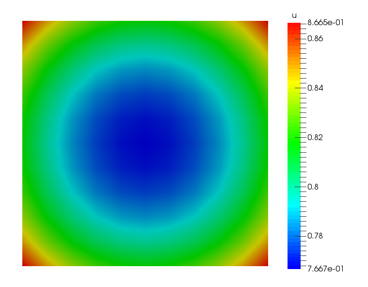
Figure 25: 拉普拉斯-杨解图
24. 网格系统
一个用于定义有限元/有限体积网格的系统。
24.1. 创建网格
对于复杂的几何形状,我们通常使用桑迪亚国家实验室的 CUBIT (cubit.sandia.gov)。
其他网格生成器只要能输出 libMesh 读取的文件格式就可以工作。
24.2. 网格生成器
MOOSE 中的网格是使用 MeshGenerators 构建或加载的。
如果只想生成网格而不运行仿真,可以在命令行上传递 –mesh-only。
24.3. FileMeshGenerator
FileMeshGenerator 是用于加载外部网格的 MeshGenerator:
[Mesh]
[fmg]
type = FileMeshGenerator
file = square.e
[]
[]
MOOSE 支持读写大量格式,并且可以扩展以读取更多格式。
24.4. 在 MOOSE 中生成网格
内置的网格生成功能实现了线、矩形、长方体或挤压反应堆几何形状的生成。
[Mesh]
[generated]
type = GeneratedMeshGenerator
dim = 2
xmin = 0
xmax = 1
nx = 2
ymin = -2
ymax = 3
ny = 3
elem_type = 'TRI3'
[]
[]
边被以逻辑方式命名和编号:
1D: left = 0, right = 1 2D: bottom = 0, right = 1, top = 2, left = 3 3D: back = 0, bottom = 1, right = 2, top = 3, left = 4, front = 5 该功能对于参数化网格优化非常方便!
24.5. 命名实体支持
可以为块、边集和节点集分配人类可读的名称,这些名称可以在整个输入文件中使用。
[Mesh]
file = three_block.e

这些名称将动态应用于网格
以便它们可以在输入文件中使用
此外,它们将显示在输出文件中
block_id = '1 2 3'
block_name = 'wood steel copper'

boundary_id = '1 2'
boundary_name = 'left right'
[]

[BCs]
active = 'left right'

[left]
type = DirichletBC
variable = u
boundary = 'left'
value = 0
[]

[right]
type = DirichletBC
variable = u
boundary = 'right'
value = 1
[]
[]

[Materials]
active = empty

[empty]
type = MTMaterial
block = 'wood steel copper'
[]
[]
需要 ID 的参数将接受数字或“名称”。
可以为现有网格的 ID 分配名称,以简化输入文件的维护。
25. 输出系统
一个用于将仿真数据输出到屏幕或文件的系统。
输出系统被设计成与 MOOSE 中的任何其他系统一样:模块化和可扩展。
可以创建多个输出对象用于输出:
在特定的时间或时间步间隔, 自定义的变量子集,以及 到各种文件类型。 对于常见的输出类型和常见参数,存在快捷语法。
25.1. 快捷语法
在 MOOSE 内部,以下两种创建 Output 对象的方法是等效的。
[Outputs]
exodus = true
[]
[Outputs]
[out]
type = Exodus
[]
[]
25.2. 自定义输出
每个 Output 的内容都可以自定义,例如,对于一个 Exodus 输出:
[Outputs]
[out]
type = Exodus
output_material_properties = true
# 从输出中移除一些量
hide = 'power_pp pressure_var'
[]
[]
25.3. 常用参数
[Outputs]
interval = 10 # 这是一个时间步间隔
[exo]
type = Exodus
interval = 1 # 覆盖顶层的 interval
[]
[cp]
type = Checkpoint # 使用顶层指定的 interval
[]
[]
25.4. 输出名称
输出文件的默认命名方案利用输入文件名(例如,input.i)和一个根据输出定义方式不同的后缀:使用快捷语法创建的 Outputs 使用 _out 后缀。子块使用实际的子块名称作为后缀。
[Outputs]
exodus = true # 创建 input_out.e
[other] # 创建 input_other.e
type = Exodus
interval = 2
[]
[base]
type = Exodus
file_base = out # 创建 out.e
[]
[]
Paraview 可以读取其中许多格式(CSV, Exodus, Nemesis, VTK, GMV)。
26. 第 3 步:带材料的压力核
使用 Material 系统提供值,而不是将常量参数传递给 DarcyPressure 对象。
[-∇ ⋅ (\frac{\mathbf{K}}{μ} ∇ p)]
其中 (\mathbf{K}) 是渗透率张量,(μ) 是流体粘度。
该系统允许属性随空间和时间变化,并可以与仿真中的变量耦合。
27. 材料系统
一个用于定义材料属性的系统,供多个系统使用并允许变量耦合。
材料系统通过在对象之间创建生产者/消费者关系来运作。
Material 对象 生产 属性。 其他 MOOSE 对象(包括材料)消费 这些属性。
27.1. 生产属性
继承自 Material 或 ADMaterial 在 validParams() 中定义参数 在构造函数中调用 declareADProperty<TYPE>("propertyname") 在 computeQpProperties() 中计算属性值
27.2. 消费属性
要消费一个材料属性,在对象中调用正确的 get 方法,并将常量引用存储为成员变量。
getMaterialProperty<TYPE>(): 在非 AD 对象内部使用,以检索非 AD 材料属性。 getADMaterialProperty<TYPE>(): 在 AD 对象内部使用,以检索 AD 材料属性。
27.3. 材料属性评估
根据需要,在求积点重新计算量。
多个 Material 对象可以为子域或边界的不同部分定义相同的“属性”。
27.4. 有状态的材料属性
除非启用了“有状态”属性,否则值不会在时间步之间存储,这是通过调用 getMaterialPropertyOld<TYPE>() 或 getMaterialPropertyOlder<TYPE>() 来实现的。
在仿真中拥有材料属性的“旧”值可能很有用,例如在固体力学塑性本构模型中。
传统上,这种类型的值被称为“状态变量”;在 MOOSE 中,它们被称为“有状态的材料属性”。
有状态的材料属性需要更多内存。
27.5. 默认材料属性
材料属性的默认值可以在 validParams 函数中分配。
addParam<MaterialPropertyName>("combination_property_name", 12345,
"The name of the property providing the luggage combination");
只有标量 (Real) 值可以有默认值。
当调用 getMaterialProperty<Real>("combinationpropertyname") 时,如果该值未通过 Material 对象内的 declareProperty 调用计算,则将返回默认值。
27.6. 材料属性输出
通过设置 outputs 参数启用材料属性的输出。
[Materials]
[block_1]
type = OutputTestMaterial
block = 1
output_properties = 'real_property tensor_property'
outputs = exodus
variable = u
[]
[block_2]
type = OutputTestMaterial
block = 2
output_properties = 'vector_property tensor_property'
outputs = exodus
variable = u
[]
[]

[Outputs]
exodus = true
[]
以下示例创建了名为 "realproperty"、"tensorproperty" 和 "vectorproperty" 的附加变量,这些变量将显示在输出文件中。
27.7. 支持输出的属性类型
材料属性可以是任意 (C++) 类型,但并非所有类型都可以输出。
Real RealVectorValue RealTensorValue
28. 函数系统
一个用于定义基于空间位置 ( x x , y y , z z ) 和时间 t t 的解析表达式的系统。
Function 对象是通过继承自 Function 并重写虚函数 value()(以及可选地其他方法)来创建的。
函数可以在大多数 MOOSE 对象中通过调用 getFunction("name") 来访问,其中 "name" 与输入文件中的名称匹配。
Function 可以依赖于其他函数,但不能依赖于材料属性或变量。
28.1. 函数使用
MOOSE 中存在许多利用函数的对象,例如:
FunctionDirichletBC FunctionNeumannBC FunctionIC BodyForce 这些对象中的每一个都有一个在输入文件中设置的 "function" 参数,用于控制使用哪个 Function 对象。
28.2. 解析函数
ParsedFunction 允许直接在输入文件中通过字符串定义函数,例如:
[Functions]
[sin_fn]
type = ParsedFunction
expression = sin(x)
[]
[cos_fn]
type = ParsedFunction
expression = cos(x)
[]
[fn]
type = ParsedFunction
expression = 's/c'
symbol_names = 's c'
symbol_values = 'sin_fn cos_fn'
[]
[]
可以包含其他函数(如上所示),以及标量变量和后处理器值与函数定义一起。
28.3. 默认函数
每当通过 addParam() 添加 Function 对象时,都可以提供一个默认值。
// 添加一个带默认常量的 Function
params.addParam<FunctionName>("pressure_grad", "0.5", "The gradient of ...");

// 添加一个带默认解析函数的 Function
params.addParam<FunctionName>("power_history", "t+100*sin(y)", "The power history of ...");
常量值和解析函数字符串都可以用作默认值。
如果输入文件中未提供函数名,则会根据默认值自动构造 ParsedFunction 或 ConstantFunction 对象。
29. 第 3 步:带材料的压力核
29.1. (续)
29.2. PackedColumn 材料
必须生产两种材料属性供 DarcyPressure 对象使用:渗透率和粘度。
两者都将由一个 Material 对象计算:PackedColumn。
与参考文献中一样,渗透率随钢球尺寸而变化,因此我们将对其在有效值范围内进行插值计算。
29.3. PackedColumn.h
#pragma once

#include "Material.h"

/**

Material 对象继承自 Material 并重写 computeQpProperties。
它们的工作是声明供其他对象(如 Kernels 和 BoundaryConditions)在计算中使用的属性。
*/
class PackedColumn : public Material
{
public:
static InputParameters validParams();
PackedColumn(const InputParameters & parameters);

protected:
/// 必要的重写。这里是计算属性值的地方。
virtual void computeQpProperties() override;

/// 柱中球体的半径
const Function & _input_radius;

/// 来自输入文件的粘度值
const Real & _input_viscosity;

/// 根据半径 (mm) 计算的渗透率 (K)
ADMaterialProperty<Real> & _permeability;

/// 流体的粘度 (mu)
ADMaterialProperty<Real> & _viscosity;
};
29.4. PackedColumn.C
#include "PackedColumn.h"
#include "Function.h"

registerMooseObject("DarcyThermoMechApp", PackedColumn);

InputParameters
PackedColumn::validParams()
{
InputParameters params = Material::validParams();

// 用于插值渗透率的球体半径参数。
params.addParam<FunctionName>("radius",
"1.0",
"The radius of the steel spheres (mm) that are packed in the "
"column for computing permeability.");
params.addParam<Real>(
"viscosity",
7.98e-4,
"The viscosity (
m
u
mu
) of the fluid in Pa, the default is for water at 30 degrees C.");

return params;
}

PackedColumn::PackedColumn(const InputParameters & parameters)
: Material(parameters),

Generated code
// 从输入文件中获取参数
_input_radius(getFunction("radius")),
_input_viscosity(getParam<Real>("viscosity")),

// 此对象生产的材料属性
_permeability(declareADProperty<Real>("permeability")),
_viscosity(declareADProperty<Real>("viscosity"))
content_copy
download
Use code with caution.
{
}

void
PackedColumn::computeQpProperties()
{
// 来自论文:表 1
std::vector<Real> sphere_sizes = {1, 3};
std::vector<Real> permeability = {0.8451e-9, 8.968e-9};

Real value = _input_radius.value(_t, _q_point[_qp]);
mooseAssert(value >= 1 && value <= 3,
"The radius range must be in the range [1, 3], but " << value << " provided.");

_viscosity[_qp] = _input_viscosity;

// 我们将使用上面两点的简单线性插值来计算渗透率:
// y0 * (x1 - x) + y1 * (x - x0)
// y(x) = -------------------------------
// x1 - x0
_permeability[_qp] =
(permeability[0] * (sphere_sizes[1] - value) + permeability[1] * (value - sphere_sizes[0])) /
(sphere_sizes[1] - sphere_sizes[0]);
}
29.5. DarcyPressure Kernel
现有的 Kernel 对象使用输入参数来定义渗透率和粘度,必须更新它以使用新创建的材料属性。
29.6. DarcyPressure.h
@@ -1,24 +1,32 @@

#pragma once

// 在这里包含 "ADKernel" Kernel 以便我们可以扩展它
#include "ADKernel.h"

/**

计算残差贡献:K / mu * grad_u * grad_phi.
*/
class DarcyPressure : public ADKernel
{
public:
static InputParameters validParams();
DarcyPressure(const InputParameters & parameters);

protected:
/// ADKernel 对象必须覆盖 precomputeQpResidual
virtual ADReal computeQpResidual() override;

/// 从输入文件设置的引用
const Real & _permeability;
const Real & _viscosity;
// 从 Material 系统设置的引用
/// 粘度。这被声明为 \p ADMaterialProperty,意味着任何来自生产 \p Material 的导数信息
/// 都将被保留,非线性求解的完整性也将同样被保留
const ADMaterialProperty<Real> & _permeability;
/// 粘度。这被声明为 \p ADMaterialProperty,意味着任何来自生产 \p Material 的导数信息
/// 都将被保留,非线性求解的完整性也将同样被保留
const ADMaterialProperty<Real> & _viscosity;
};
29.7. DarcyPressure.C
@@ -1,37 +1,26 @@

#include "DarcyPressure.h"

registerMooseObject("DarcyThermoMechApp", DarcyPressure);

InputParameters
DarcyPressure::validParams()
{
InputParameters params = ADKernel::validParams();
params.addClassDescription("Compute the diffusion term for Darcy pressure (
p
p
) equation: "
"
−
n
a
b
l
a
c
d
o
t
f
r
a
c
m
a
t
h
b
f
K
m
u
n
a
b
l
a
p
=
0
−
nabla
cdot
fracmathbfKmu
nablap=0
");
// 添加一个必需的参数。如果输入文件中未提供此参数,MOOSE 将会报错。
params.addRequiredParam<Real>("permeability", "The permeability (
m
a
t
h
r
m
K
mathrmK
) of the fluid.");
// 添加一个带默认值的参数;此值可以在输入文件中覆盖。
params.addParam<Real>(
Generated code
"viscosity",
content_copy
download
Use code with caution.
Generated code
7.98e-4,
content_copy
download
Use code with caution.
Generated code
"The viscosity ($\\mu$) of the fluid in Pa, the default is for water at 30 degrees C.");
content_copy
download
Use code with caution.
return params;
}
DarcyPressure::DarcyPressure(const InputParameters & parameters)
: ADKernel(parameters),
// 从输入文件中获取参数
_permeability(getParam<Real>("permeability")),
_viscosity(getParam<Real>("viscosity"))
_permeability(getADMaterialProperty<Real>("permeability")),
_viscosity(getADMaterialProperty<Real>("viscosity"))
{
}
ADReal
DarcyPressure::computeQpResidual()
{

return (_permeability / _viscosity) * _grad_test[_i][_qp] * _grad_u[_qp];
return (_permeability[_qp] / _viscosity[_qp]) * _grad_test[_i][_qp] * _grad_u[_qp];
}
29.8. 第 3 步:输入文件
@@ -1,52 +1,55 @@
[Mesh]
[gmg]

type = GeneratedMeshGenerator # Can generate simple lines, rectangles and rectangular prisms
dim = 2 # Dimension of the mesh
nx = 100 # Number of elements in the x direction
ny = 10 # Number of elements in the y direction
xmax = 0.304 # Length of test chamber
ymax = 0.0257 # Test chamber radius
type = GeneratedMeshGenerator
dim = 2
nx = 100
ny = 10
xmax = 0.304
ymax = 0.0257
[]
coord_type = RZ # Axisymmetric RZ
rz_coord_axis = X # Which axis the symmetry is around
coord_type = RZ
rz_coord_axis = X
[]
[Variables/pressure]

Adds a Linear Lagrange variable by default
[]

[Kernels/darcy_pressure]
type = DarcyPressure
variable = pressure
-- permeability = 0.8451e-9 # (m^2) 1mm spheres.
[]

[BCs]
[inlet]

type = DirichletBC # Simple u=value BC
variable = pressure # Variable to be set
boundary = left # Name of a sideset in the mesh
value = 4000 # (Pa) From Figure 2 from paper. First data point for 1mm spheres.
type = DirichletBC
variable = pressure
boundary = left
value = 4000
[]
[outlet]
type = DirichletBC<<<{"description": "Imposes the essential boundary condition
u
=
g
u=g
, where
g
g
 is a constant, controllable value.", "href": "../source/bcs/DirichletBC.html"}>>>
variable<<<{"description": "The name of the variable that this residual object operates on"}>>> = pressure
boundary<<<{"description": "The list of boundary IDs from the mesh where this object applies"}>>> = right
value<<<{"description": "Value of the BC"}>>> = 0 # (Pa) Gives the correct pressure drop from Figure 2 for 1mm spheres
type = DirichletBC
variable = pressure
boundary = right
value = 0
[]
[]
+[Materials/column]

type = PackedColumn
+[]
[Problem]

type = FEProblem # This is the "normal" type of Finite Element Problem in MOOSE
type = FEProblem
[]
[Executioner]

type = Steady # Steady state problem
solve_type = NEWTON # Perform a Newton solve, uses AD to compute Jacobian terms
petsc_options_iname = '-pc_type -pc_hypre_type' # PETSc option pairs with values below
type = Steady
solve_type = NEWTON
petsc_options_iname = '-pc_type -pc_hypre_type'
petsc_options_value = 'hypre boomeramg'
[]
[Outputs]

exodus<<<{"description": "Output the results using the default settings for Exodus output."}>>> = true # Output Exodus format
exodus = true
[]
29.9. 第 3 步:运行
cd ~/projects/moose/tutorials/darcy_thermo_mech/step03_darcy_material
make -j 12 # 使用您系统的处理器数量
cd problems
../darcy_thermo_mech-opt -i step3.i
29.10. 第 3 步:结果

Figure 26: 第 3 步结果图
29.11. 第 3b 步:可变球体
更新输入文件,使球体尺寸沿管道长度从 1 变化到 3。
29.12. 第 3b 步:输入文件
@@ -1,55 +1,57 @@
[Mesh]
[gmg]

type = GeneratedMeshGenerator # Can generate simple lines, rectangles and rectangular prisms
dim = 2 # Dimension of the mesh
nx = 100 # Number of elements in the x direction
ny = 10 # Number of elements in the y direction
xmax = 0.304 # Length of test chamber
ymax = 0.0257 # Test chamber radius
type = GeneratedMeshGenerator
dim = 2
nx = 100
ny = 10
xmax = 0.304
ymax = 0.0257
[]
coord_type = RZ # Axisymmetric RZ
rz_coord_axis = X # Which axis the symmetry is around
coord_type = RZ
rz_coord_axis = X
[]
[Variables/pressure]

Adds a Linear Lagrange variable by default
[]

[Kernels/darcy_pressure]
type = DarcyPressure
variable = pressure
[]

[BCs]
[inlet]

type = DirichletBC # Simple u=value BC
variable = pressure # Variable to be set
boundary = left # Name of a sideset in the mesh
value = 4000 # (Pa) From Figure 2 from paper. First data point for 1mm spheres.
type = DirichletBC
variable = pressure
boundary = left
value = 4000
[]
[outlet]
type = DirichletBC<<<{"description": "Imposes the essential boundary condition
u
=
g
u=g
, where
g
g
 is a constant, controllable value.", "href": "../source/bcs/DirichletBC.html"}>>>
variable<<<{"description": "The name of the variable that this residual object operates on"}>>> = pressure
boundary<<<{"description": "The list of boundary IDs from the mesh where this object applies"}>>> = right
value<<<{"description": "Value of the BC"}>>> = 0 # (Pa) Gives the correct pressure drop from Figure 2 for 1mm spheres
type = DirichletBC
variable = pressure
boundary = right
value = 0
[]
[]
[Materials/column]
type = PackedColumn
-+ radius = '1 + 2/3.04x'
++ radius = '1 + 2/0.304x'

outputs = exodus
[]
[Problem]

type = FEProblem # This is the "normal" type of Finite Element Problem in MOOSE
type = FEProblem
[]
[Executioner]

type = Steady # Steady state problem
solve_type = NEWTON # Perform a Newton solve, uses AD to compute Jacobian terms
petsc_options_iname = '-pc_type -pc_hypre_type' # PETSc option pairs with values below
type = Steady
solve_type = NEWTON
petsc_options_iname = '-pc_type -pc_hypre_type'
petsc_options_value = 'hypre boomeramg'
[]
[Outputs]

exodus<<<{"description": "Output the results using the default settings for Exodus output."}>>> = true # Output Exodus format
exodus = true
[]
29.13. 第 3b 步:结果
Figure 27: 第 3b 步结果图
30. 测试系统
30.1. 持续集成
持续集成是一种软件开发实践,开发人员定期将其代码更改合并到中央仓库中,然后运行自动化的构建和测试。持续集成的关键目标是更快地发现和解决错误,提高软件质量,并减少验证和发布新软件更新所需的时间。
测试通过确保您的更改不会破坏代码以前的功能来实现持续集成。
30.2. 概述
MOOSE 包含一个可扩展的测试系统 (python),用于使用不同的输入文件执行代码。
每个内核(或一组逻辑内核)都应该有用于验证的测试。
测试系统是灵活的,它执行许多不同的操作,例如测试预期的错误条件。
此外,可以创建自定义的 "Tester" 对象。
30.3. 测试设置
相关测试应分组到单个目录中,并具有一致的命名约定。
建议以与应用程序源类似的层次结构组织测试(即内核、BC、材料等)。
通过匹配模式(如下突出显示)动态查找测试。
tests/
kernels/
my_kernel_test/
my_kernel_test.e [输入网格]
my_kernel_test.i [输入文件]
tests [测试规范文件]
gold/ [用于验证解的黄金标准文件夹]
out.e [解]
30.4. 测试规范
测试规范使用 hit 格式,与标准 MOOSE 输入文件格式相同。
[Tests]
[my_kernel_test]
type = Exodiff
input = my_kernel_test.i
exodiff = my_kernel_test_out.e
[]

[kernel_check_exception]
type = RunException
input = my_kernel_exception.i
expect_err = 'Bad stuff happened with variable \w+'
[]
[]
30.5. 测试对象
RunApp: 使用指定选项运行基于 MOOSE 的应用程序 Exodiff: 检查 Exodus 文件是否存在指定公差内的差异 CSVDiff: 检查 CSV 文件是否存在指定公差内的差异 VTKDiff: 检查 VTK 文件是否存在指定公差内的差异 RunException: 测试错误条件 CheckFiles: 检查已完成运行后是否存在特定文件 ImageDiff: 比较图像(例如 *.png)是否存在指定公差内的差异 PythonUnitTest: 运行基于 python "unittest" 的测试 AnalyzeJacobian: 将计算出的雅可比与有限差分版本进行比较 PetscJacobianTester: 使用 PETSc 比较计算出的雅可比
30.6. 运行测试
./run_tests -j 12
要获取更多信息,请查看帮助:
./run_tests -h
30.7. 测试对象选项
input: 输入文件的名称 exodiff: 要比较的输出文件名列表 abszero: exodiff 的绝对零容差 relerr: exodiff 的相对误差容差 prereq: 在运行此测试之前需要完成的测试名称 minparallel: 用于测试的最小处理器数(默认值:1) maxparallel: 用于测试的最大处理器数
./run_tests --dump
30.8. 关于测试的说明
单个测试应相对较快地运行(2 秒规则)。
输出或其他生成的文件不应检入仓库。
MOOSE 开发人员在重构时依赖于应用程序测试来验证正确性。
测试覆盖率差 = 代码故障率高
31. 第 4 步:速度辅助变量
速度是主要关注的变量,它根据压力计算得出:
[\mathbf{v} = -\frac{\mathbf{K}}{μf} ∇ p]
32. 辅助系统
一个用于直接计算场变量(“AuxVariables”)的系统,设计用于后处理、耦合和代理计算。
术语“非线性变量”在 MOOSE 语言中定义为使用 Kernel 和 BoundaryCondition 对象通过非线性 PDE 系统求解的变量。
术语“辅助变量”在 MOOSE 语言中定义为使用 AuxKernel 对象直接计算的变量。
32.1. AuxVariables
辅助变量在 [AuxVariables] 输入文件块中声明。
辅助变量是与有限元形函数关联的场变量,可以作为非线性变量的代理。
辅助变量目前有两种类型:
单元(例如,常数或高阶单项式) 节点(例如,线性拉格朗日) 辅助变量具有“旧”和“更旧”的状态,来自先前的时间步,就像非线性变量一样。
32.1.1. 单元辅助变量
单元辅助变量可以计算:
每个单元的平均值,如果存储在常数单项式变量中 使用高阶变量的空间分布
[AuxVariables]
[aux]
order = CONSTANT
family = MONOMIAL
[]
[]
计算单元值的 AuxKernel 对象可以耦合到非线性变量以及单元和节点辅助变量。
32.1.2. 节点辅助变量
节点辅助变量在每个节点计算,并存储为线性拉格朗日变量。
[AuxVariables]
[aux]
order = LAGRANGE
family = FIRST
[]
[]
计算节点值的 AuxKernel 对象只能耦合到节点非线性变量和其他节点辅助变量。
32.2. AuxKernel 对象
通过重写 computeValue() 直接计算 AuxVariable 值,它们可以对单元和节点辅助变量进行操作。
当对节点变量进行操作时,computeValue() 对每个节点进行操作;当对单元变量进行操作时,它对每个单元进行操作。
32.3. AuxKernel 对象成员
_u, _gradu: 此 AuxKernel 操作的变量的值和梯度 _qpoint: 当前 q 点的坐标,仅对单元 AuxKernels 有效,对于节点变量应使用 _currentnode _qp: 当前求积点,此索引用于节点(在节点处 _qp=0)和单元变量以保持一致性 _currentelem: 指向当前操作的单元的指针(仅限单元) _currentnode: 指向当前操作的节点的指针(仅限节点)
32.4. VectorAuxKernel 对象
通过以下方式直接计算向量 AuxVariable 值:
继承自 VectorAuxKernel 类 重写 computeValue(),不同之处在于返回值是 RealVectorValue 而不是 Real。
[AuxVariables]
[aux]
order = FIRST
family = LAGRANGE_VEC
[]
[]
[AuxKernels]
[parsed]
type = ParsedVectorAux
variable = aux
expression_x = 'x + y'
expression_y = 'x - y'
[]
[]
辅助变量必须是向量类型之一(LAGRANCEVEC、MONOMIALVEC 或 NEDELECVEC)。
33. 第 4 步:速度辅助变量
33.1. (续)
33.2. DarcyVelocity AuxKernel
主要未知数(“非线性变量”)是压力 (→ \mathbf{v})。
一旦计算出压力,AuxiliarySystem 就可以使用耦合的压力变量以及渗透率和粘度属性来计算和输出速度场。
辅助变量有两种类型:节点型和单元型。
节点辅助变量不能耦合到非线性变量的梯度,因为连续变量的梯度在节点上没有明确定义。 单元辅助变量可以耦合到非线性变量的梯度,因为求值发生在单元内部。
33.3. DarcyVelocity.h
#pragma once

#include "AuxKernel.h"

/**

辅助内核,负责在给定多种流体属性和压力梯度的情况下计算达西速度。
*/
class DarcyVelocity : public VectorAuxKernel
{
public:
static InputParameters validParams();
DarcyVelocity(const InputParameters & parameters);

protected:
/**

AuxKernels 必须重写 computeValue。computeValue() 在每个求积点上被调用。
对于节点辅助变量,这些求积点与节点重合。
*/
virtual RealVectorValue computeValue() override;
/// 耦合变量的梯度
const VariableGradient & _pressure_gradient;

/// 保存来自材料系统的渗透率和粘度
const ADMaterialProperty<Real> & _permeability;
const ADMaterialProperty<Real> & _viscosity;
};
33.4. DarcyVelocity.C
#include "DarcyVelocity.h"

#include "metaphysicl/raw_type.h"

registerMooseObject("DarcyThermoMechApp", DarcyVelocity);

InputParameters
DarcyVelocity::validParams()
{
InputParameters params = VectorAuxKernel::validParams();

// 添加一个“耦合参数”以从输入文件中获取一个变量。
params.addRequiredCoupledVar("pressure", "The pressure field.");

return params;
}

DarcyVelocity::DarcyVelocity(const InputParameters & parameters)
: VectorAuxKernel(parameters),

Generated code
// 获取变量的梯度
_pressure_gradient(coupledGradient("pressure")),

// 设置对渗透率 MaterialProperty 的引用。
// 只有作用于单元辅助变量的 AuxKernels 才能这样做
_permeability(getADMaterialProperty<Real>("permeability")),

// 设置对粘度 MaterialProperty 的引用。
// 只有作用于单元辅助变量的 AuxKernels 才能这样做
_viscosity(getADMaterialProperty<Real>("viscosity"))
content_copy
download
Use code with caution.
{
}

RealVectorValue
DarcyVelocity::computeValue()
{
// 访问此求积点处的压力梯度,然后提取其请求的“分量”(x、y 或 z)。
// 注意,获取梯度的特定分量是使用括号运算符完成的。
return -MetaPhysicL::raw_value(_permeability[_qp] / _viscosity[_qp]) * _pressure_gradient[_qp];
}
33.5. 第 4 步:输入文件
@@ -1,55 +1,70 @@
[Mesh]
[gmg]

type = GeneratedMeshGenerator # Can generate simple lines, rectangles and rectangular prisms
dim = 2 # Dimension of the mesh
nx = 100 # Number of elements in the x direction
ny = 10 # Number of elements in the y direction
xmax = 0.304 # Length of test chamber
ymax = 0.0257 # Test chamber radius
type = GeneratedMeshGenerator
dim = 2
nx = 100
ny = 10
xmax = 0.304
ymax = 0.0257
[]
coord_type = RZ # Axisymmetric RZ
rz_coord_axis = X # Which axis the symmetry is around
coord_type = RZ
rz_coord_axis = X
[]
[Variables/pressure]

Adds a Linear Lagrange variable by default
[]

+[AuxVariables/velocity]

order = CONSTANT
family = MONOMIAL_VEC
+[]
[Kernels/darcy_pressure]
type = DarcyPressure
variable = pressure
+[]
+
+[AuxKernels]

[velocity]
type = DarcyVelocity
variable = velocity
execute_on = timestep_end
pressure = pressure
[]
[]
[BCs]
[inlet]

type = DirichletBC # Simple u=value BC
variable = pressure # Variable to be set
boundary = left # Name of a sideset in the mesh
value = 4000 # (Pa) From Figure 2 from paper. First data point for 1mm spheres.
type = DirichletBC
variable = pressure
boundary = left
value = 4000
[]
[outlet]
type = DirichletBC<<<{"description": "Imposes the essential boundary condition
u
=
g
u=g
, where
g
g
 is a constant, controllable value.", "href": "../source/bcs/DirichletBC.html"}>>>
variable<<<{"description": "The name of the variable that this residual object operates on"}>>> = pressure
boundary<<<{"description": "The list of boundary IDs from the mesh where this object applies"}>>> = right
value<<<{"description": "Value of the BC"}>>> = 0 # (Pa) Gives the correct pressure drop from Figure 2 for 1mm spheres
type = DirichletBC
variable = pressure
boundary = right
value = 0
[]
[]
[Materials/column]
type = PackedColumn

radius = 1
[]
[Problem]

type = FEProblem # This is the "normal" type of Finite Element Problem in MOOSE
type = FEProblem
[]
[Executioner]

type = Steady # Steady state problem
solve_type = NEWTON # Perform a Newton solve, uses AD to compute Jacobian terms
petsc_options_iname = '-pc_type -pc_hypre_type' # PETSc option pairs with values below
type = Steady
solve_type = NEWTON
petsc_options_iname = '-pc_type -pc_hypre_type'
petsc_options_value = 'hypre boomeramg'
[]
[Outputs]

exodus<<<{"description": "Output the results using the default settings for Exodus output."}>>> = true # Output Exodus format
exodus = true
[]
33.6. 第 4 步:运行
cd ~/projects/moose/tutorials/darcy_thermo_mech/step04_velocity_aux
make -j 12 # 使用您系统的处理器数量
cd problems
../darcy_thermo_mech-opt -i step4.i
33.7. 第 4 步:结果

Figure 28: 第 4 步结果图
33.8. 更紧的求解公差

Figure 29: 第 4 步结果图(更紧公差)
cd ~/projects/moose/tutorials/darcy_thermo_mech/step04_velocity_aux
make -j 12 # 使用您系统的处理器数量
cd problems
../darcy_thermo_mech-opt -i step4.i Executioner/nl_rel_tol=1e-12
34. 第 5 步:热传导
处理完压力方程后,接下来是热传导方程。
[(ρ cp)m \frac{\partial T}{\partial t} + (ρ cp)f \mathbf{v} ⋅ ∇ T - ∇ ⋅ (km ∇ T) = 0]
最初,只考虑稳态热传导方程:
[-∇ ⋅ (km ∇ T) = 0]
这是另一个扩散型项,它依赖于导热系数 k m k m
。该项在 MOOSE 热传递模块中实现为 ADHeatConduction。
34.1. ADHeatConduction.h
#pragma once

#include "ADDiffusion.h"

class ADHeatConduction : public ADDiffusion
{
public:
static InputParameters validParams();

ADHeatConduction(const InputParameters & parameters);

protected:
virtual ADRealVectorValue precomputeQpResidual() override;

const ADMaterialProperty<Real> & _thermal_conductivity;
};
34.2. ADHeatConduction.C
#include "ADHeatConduction.h"

registerMooseObject("HeatTransferApp", ADHeatConduction);

InputParameters
ADHeatConduction::validParams()
{
InputParameters params = ADDiffusion::validParams();
params.addParam<MaterialPropertyName>("thermal_conductivity",
"thermal_conductivity",
"the name of the thermal conductivity material property");
params.set<bool>("use_displaced_mesh") = true;
return params;
}

ADHeatConduction::ADHeatConduction(const InputParameters & parameters)
: ADDiffusion(parameters),
_thermal_conductivity(getADMaterialProperty<Real>("thermal_conductivity"))
{
}

ADRealVectorValue
ADHeatConduction::precomputeQpResidual()
{
return _thermal_conductivity[_qp] * ADDiffusion::precomputeQpResidual();
}
ADHeatConduction Kernel 与 GenericConstantMaterial 结合使用,足以进行稳态热传导求解(入口处 T = 350 T=350 ,出口处 T = 300 T=300 )。
34.3. GenericConstantMaterial
GenericConstantMaterial 是定义常数材料属性的一种简单方法。
[Materials/material]
type = GenericConstantMaterial
prop_names = 'conductivity density'
prop_values = '0.01 200'
[]
使用 MOOSE 中常见的“列表”语法提供了两个输入参数:propnames 和 propvalues。
34.4. 第 5a 步:稳态输入文件
[Mesh]
[gmg]
type = GeneratedMeshGenerator
dim = 2
nx = 100
ny = 10
xmax = 0.304 # 测试室长度
ymax = 0.0257 # 测试室半径
[]
coord_type = RZ
rz_coord_axis = X
[]

[Variables]
[temperature]
[]
[]

[Kernels]
[heat_conduction]
type = ADHeatConduction
variable = temperature
[]
[]

[BCs]
[inlet_temperature]
type = DirichletBC
variable = temperature
boundary = left
value = 350 # (K)
[]
[outlet_temperature]
type = DirichletBC
variable = temperature
boundary = right
value = 300 # (K)
[]
[]

[Materials/steel]
type = ADGenericConstantMaterial
prop_names = thermal_conductivity
prop_values = 18 # K: (W/m*K) 来自维基百科 @296K
[]

[Problem]
type = FEProblem
[]

[Executioner]
type = Steady
solve_type = NEWTON
petsc_options_iname = '-pc_type -pc_hypre_type'
petsc_options_value = 'hypre boomeramg'
[]

[Outputs]
exodus = true
[]
34.5. 第 5a 步:运行输入文件
cd ~/projects/moose/tutorials/darcy_thermo_mech/step5_heat_conduction
make -j 12 # 使用您系统的处理器数量
cd problems
../darcy_thermo_mech-opt -i step5a_steady.i
34.6. 瞬态热传导 (5b)
要创建一个时间相关的问题,需要加入时间导数项:
[ρm cpm \frac{\partial T}{\partial t}]
时间项存在于热传递模块的 ADHeatConductionTimeDerivative 中,因此只需要更新输入文件即可运行瞬态情况。
35. Executioner 系统
一个用于指定仿真求解策略的系统。
35.1. 稳态 Executioner
稳态执行器通常只求解非线性系统一次。
[Executioner]
type = Steady
[]
Steady 执行器可以在自适应细化网格以改善解的同时多次求解非线性系统。
35.2. 瞬态 Executioners
瞬态执行器在每个时间步至少求解一次非线性系统。
[Executioner]
type = Transient
scheme = 'implicit-euler'
solve_type = 'PJFNK'
start_time = 0.0
num_steps = 5
dt = 0.1
[]
35.2.1. 稳态检测
如果连续 N 个时间步的解没有显著变化,瞬态仿真可以提前终止。 对于稳态问题,这可以用于在自适应网格细化之间获得更好的初始猜测。
35.3. 常见 Executioner 选项
type: Steady, Transient solvetype: PJFNK, JFNK, NEWTON, FD petscoptionsiname/value: PETSc 选项 nlabstol/nlreltol: 非线性绝对/相对容差 labstol/lreltol: 线性绝对/相对容差 starttime/endtime: 开始/结束时间 dt/dtmin/dtmax: 时间步长/最小/最大 numsteps: 时间步数
35.4. TimeKernel 对象
TimeKernel 对象向 Kernel 对象添加了两个成员变量:
_udot: 相关非线性变量的时间导数 _dudotdu: _udot 相对于 _u 的导数
35.5. TimeKernel 基类
TimeKernel: 手动雅可比 ADTimeKernel: 自动微分
36. 时间积分器系统
一个用于定义时间数值积分方案的系统。
TimeIntegrator 可以在 [Executioner] 块中使用 "scheme" 参数设置,如果 "type = Transient",则存在以下选项:
implicit-euler: 后向欧拉(默认) bdf2: 二阶后向差分公式 crank-nicolson: 二阶 Crank-Nicolson 方法 dirk: 二阶对角隐式龙格-库塔 (DIRK) newmark-beta: 二阶 Newmark-beta 方法(结构动力学)
36.1. TimeIntegrator 块
也可以将时间积分器指定为输入文件中的一个单独子块。这允许定义其他类型和参数,包括自定义的 TimeIntegrator 对象。
[Executioner]
type = Transient
start_time = 0.0
num_steps = 6
dt = 0.1
[TimeIntegrator]
type = NewmarkBeta
beta = 0.4225
gamma = 0.8
[]
[]
36.2. 收敛率
考虑测试问题:
[ut - uxx = f \quad ∀ (x, t) ∈ (0, L) × (0, T]]
对于 x ∈ [ 0 , L ] x∈[0,L] 和 t ∈ [ 0 , T ] t∈[0,T] , f ( x , t ) f(x,t) 的选择使得精确解由 u ( x , t ) = sin ( 2 π x L ) cos ( t ) u(x,t)=sin( L 2πx )cos(t) 给出, u ( x , 0 ) u(x,0) 和 u ( 0 , t ) , u ( L , t ) u(0,t),u(L,t) 是与此精确解相对应的初始和狄利克雷边界条件。

Figure 30: 时间收敛隐式欧拉
37. 时间步进器系统
一个为瞬态执行器建议时间步的系统。
自定义对象通过继承自 TimeStepper 并重写 computeDT() 来创建。
[Executioner]
type = Transient
end_time = 20.0
verbose = true

[TimeStepper]
type = IterationAdaptiveDT
dt = 1.0
optimal_iterations = 10
time_t = '0.0 5.0'
time_dt = '1.0 5.0'
[]
[]
37.1. 内置 TimeSteppers
MOOSE 包含许多内置的 TimeStepper 对象:
ConstantDT IterationAdaptiveDT FunctionDT PostprocessorDT FixedPointIterationAdaptiveDT TimeSequenceStepper
37.2. IterationAdaptiveDT
IterationAdaptiveDT 根据在上一个收敛步骤中获得收敛解所花费的迭代次数来增大或减小时间步长。
[Executioner]
type = Transient
solve_type = NEWTON
start_time = 0.0
dtmin = 1.0
end_time = 10.0
[TimeStepper]
type = IterationAdaptiveDT
optimal_iterations = 1
linear_iteration_ratio = 1
dt = 5.0
[]
[]
37.3. TimeSequenceStepper
使用参数 timesequence 提供一个时间点向量,对象只需按顺序遍历这些时间点。
starttime 和 endtime 参数会自动添加到序列中。
只考虑满足 t i ≥ t c u r r e n t t i ≥t current
的时间点。
如果求解在步骤 t i t i
失败,则会插入一个额外的时间点 t i − 1
( t i − t i − 1 ) / 2 t i−1 +(t i −t i−1 )/2 并重新求解该步骤。
37.4. 组合 TimeSteppers
现在可以组合时间步进器以遵循复杂的时间历史。默认情况下,将使用所有时间步进器计算出的所有时间步中的最小值!
[TimeSteppers]
[constant]
type = ConstantDT
dt = 0.2
[]
[hit_these_times]
type = TimeSequenceStepper
time_sequence = '0.5 1 1.5 2.1'
[]
[]
从时间 = 0s 开始,将采取哪些步骤?
0.2, 0.4, 0.5, 0.7, 0.9, 1.0, 1.2, 1.4, 1.5, 1.7, 1.9, 2.1
38. 第 5 步:热传导
38.1. (续)
38.2. 瞬态热传导 (5b)
要创建一个时间相关的问题,需要加入时间导数项:
[ρm cpm \frac{\partial T}{\partial t}]
时间项存在于热传递模块的 ADHeatConductionTimeDerivative 中,因此只需要更新输入文件即可运行瞬态情况。
38.3. ADHeatConductionTimeDerivative.h
#pragma once

#include "ADTimeDerivative.h"

class ADHeatConductionTimeDerivative : public ADTimeDerivative
{
public:
static InputParameters validParams();

ADHeatConductionTimeDerivative(const InputParameters & parameters);

protected:
virtual ADReal precomputeQpResidual() override;

/// Specific heat material property
const ADMaterialProperty<Real> & _specific_heat;

/// Density material property
const ADMaterialProperty<Real> & _density;
};
38.4. ADHeatConductionTimeDerivative.C
#include "ADHeatConductionTimeDerivative.h" registerMooseObject("HeatTransferApp", ADHeatConductionTimeDerivative); InputParameters ADHeatConductionTimeDerivative::validParams() { InputParameters params = ADTimeDerivative::validParams(); params.addClassDescription( "AD Time derivative term r h o c p f r a c p a r t i a l T p a r t i a l t rhoc p fracpartialTpartialt of " "the heat equation for quasi-constant specific heat c p c p and the density r h o rho ."); params.set<bool>("use_displaced_mesh") = true; params.addParam<MaterialPropertyName>( "specific_heat", "specific_heat", "Property name of the specific heat material property"); params.addParam<MaterialPropertyName>( "density_name", "density", "Property name of the density material property"); return params; } ADHeatConductionTimeDerivative::ADHeatConductionTimeDerivative(const InputParameters & parameters) : ADTimeDerivative(parameters), _specific_heat(getADMaterialProperty<Real>("specific_heat")), _density(getADMaterialProperty<Real>("density_name")) { } ADReal ADHeatConductionTimeDerivative::precomputeQpResidual() { return _specific_heat[_qp] * _density[_qp] * ADTimeDerivative::precomputeQpResidual(); }
38.5. 第 5b 步:时间相关的输入文件
@@ -1,60 +1,68 @@
[Mesh]
[gmg]
type = GeneratedMeshGenerator
dim = 2
nx = 100
ny = 10
xmax = 0.304 # Length of test chamber
ymax = 0.0257 # Test chamber radius
[]
coord_type = RZ
rz_coord_axis = X
[]

[Variables]
[temperature]

initial_condition = 300 # Start at room temperature
[]
[]
[Kernels]
[heat_conduction]

type = ADHeatConduction
variable = temperature
type = ADHeatConduction
variable = temperature
[]
[heat_conduction_time_derivative]
type = ADHeatConductionTimeDerivative
variable = temperature
specific_heat = specific_heat
density_name = density
[]
[]
[BCs]
[inlet_temperature]

type = DirichletBC
variable = temperature
boundary = left
value = 350 # (K)
type = DirichletBC
variable = temperature
boundary = left
value = 350
[]
[outlet_temperature]
type = DirichletBC
variable = temperature
boundary = right
value = 300 # (K)
type = DirichletBC
variable = temperature
boundary = right
value = 300
[]
[]
[Materials/steel]

type = ADGenericConstantMaterial
-- prop_names = thermal_conductivity
-- prop_values = 18 # K: (W/m*K) from wikipedia @296K
type = ADGenericConstantMaterial
prop_names = 'thermal_conductivity specific_heat density'
prop_values = '18 0.466 8000' # W/m*K, J/kg-K, kg/m^3 @ 296K
[]
[Problem]
type = FEProblem
[]

[Executioner]
-- type = Steady

type = Transient
num_steps = 10
solve_type = NEWTON
petsc_options_iname = '-pc_type -pc_hypre_type'
petsc_options_value = 'hypre boomeramg'
[]
[Outputs]

exodus = true
exodus = true
[]
38.6. 第 5b 步:运行输入文件
cd ~/projects/moose/tutorials/darcy_thermo_mech/step5_heat_conduction
make -j 12 # 使用您系统的处理器数量
cd problems
../darcy_thermo_mech-opt -i step5b_transient.i
38.7. 出流边界条件 (5c)
假设流体从管道流出到一个大水箱中,这可以用 Griffiths (1997) 的“无边界条件”边界条件来建模。
边界项 (-⟨ ψi, k ∇ T ⋅ \mathbf{n} ⟩) 是隐式计算的,而不是像在 NeumannBC 中那样用已知的通量替换。
39. 边界条件系统
用于计算 PDE 边界项残差贡献的系统。
BoundaryCondition (BC) 对象计算域边界(或内侧)上的残差。
BC 对象有两种类型:节点型和积分型。
39.1. 积分型 BC
积分型 BC 在边界或内侧上积分,应继承自 ADIntegratedBC。
其结构与 Kernels 非常相似:对象必须重写 computeQpResidual。
39.2. ADIntegratedBC 对象成员
_u, _gradu: 此 Kernel 操作的变量的值和梯度 _test, _gradtest: 求积点处的测试函数 (ψi) 的值和梯度 (∇ψi) _phi, _gradphi: 求积点处的试探函数 (φj) 的值和梯度 (∇φj) _i, _j, _qp: 分别是测试函数、试探函数和求积点的当前索引 _normals: 边界单元的外法线向量 _boundaryid: 边界 ID _currentelem, _currentside: 指向当前边界侧的单元和索引的指针
39.3. 非积分型 BC
非积分型 BC 直接在边界或内侧上设置残差值,应继承自 ADNodalBC。
其结构与 Kernels 非常相似:对象必须重写 computeQpResidual。
39.4. NodalBC 对象成员
_u: 此 Kernel 操作的变量的值 _qp: 当前索引,用于接口一致性 _boundaryid: 边界 ID _currentnode: 指向当前操作的节点的指针。
39.5. 狄利克雷 BCs
在边界上设置变量 值 的条件:
[uh = g \quad \text{on} \quad ∂Ω]
变为
[Ri = ui - gi]
39.6. DirichletBC.h
#pragma once

#include "DirichletBCBase.h"

/**

Boundary condition of a Dirichlet type
Sets the value in the node
*/
class DirichletBC : public DirichletBCBase
{
public:
static InputParameters validParams();
DirichletBC(const InputParameters & parameters);

protected:
virtual Real computeQpValue() override;

/// The value for this BC
const Real & _value;
};
39.7. DirichletBC.C
#include "DirichletBC.h"

registerMooseObject("MooseApp", DirichletBC);

InputParameters
DirichletBC::validParams()
{
InputParameters params = DirichletBCBase::validParams();
params.addRequiredParam<Real>("value", "Value of the BC");
params.declareControllable("value");
params.addClassDescription("Imposes the essential boundary condition
u
=
g
u=g
, where
g
g
 "
"is a constant, controllable value.");
return params;
}

DirichletBC::DirichletBC(const InputParameters & parameters)
: DirichletBCBase(parameters), _value(getParam<Real>("value"))
{
}

Real
DirichletBC::computeQpValue()
{
return _value;
}
39.8. 积分型 BCs
积分型 BCs(包括诺伊曼 BCs)实际上是在单元的外表面上积分的。
[⟨ ψi, ∇ u ⋅ \mathbf{n} ⟩ = 0]
变为:
[⟨ ψi, g ⟩]
如果 g = 0 g=0 ,则边界积分为零(“自然边界条件”)。
39.9. NeumannBC.h
#pragma once

#include "GenericIntegratedBC.h"

/**

Implements a simple constant Neumann BC where grad(u)=value on the boundary.
Uses the term produced from integrating the diffusion operator by parts.
*/
template <bool is_ad>
class NeumannBCTempl : public GenericIntegratedBC<is_ad>
{
public:
static InputParameters validParams();
NeumannBCTempl(const InputParameters & parameters);

protected:
virtual GenericReal<is_ad> computeQpResidual() override;

/// Value of grad(u) on the boundary.
const Real & _value;

usingGenericIntegratedBCMembers;
};

typedef NeumannBCTempl<false> NeumannBC;
typedef NeumannBCTempl<true> ADNeumannBC;
39.10. NeumannBC.C
#include "NeumannBC.h"

registerMooseObject("MooseApp", NeumannBC);
registerMooseObject("MooseApp", ADNeumannBC);

template <bool is_ad>
InputParameters
NeumannBCTempl<is_ad>::validParams()
{
InputParameters params = GenericIntegratedBC<is_ad>::validParams();
params.addParam<Real>("value",
0.0,
"For a Laplacian problem, the value of the gradient dotted with the "
"normals on the boundary.");
params.declareControllable("value");
params.addClassDescription("Imposes the integrated boundary condition "
"
f
r
a
c
p
a
r
t
i
a
l
u
p
a
r
t
i
a
l
n
=
h
fracpartialupartialn=h
, "
"where
h
h
 is a constant, controllable value.");
return params;
}

template <bool is_ad>
NeumannBCTempl<is_ad>::NeumannBCTempl(const InputParameters & parameters)
: GenericIntegratedBC<is_ad>(parameters), _value(this->template getParam<Real>("value"))
{
}

template <bool is_ad>
GenericReal<is_ad>
NeumannBCTempl<is_ad>::computeQpResidual()
{
return -_test[_i][_qp] * _value;
}

template class NeumannBCTempl<false>;
template class NeumannBCTempl<true>;
39.11. 周期性 BCs
周期性边界条件对于模拟准无限域和具有守恒量的系统非常有用。
1D、2D 和 3D 支持网格自适应 可以限制到特定变量 支持任意平移向量来定义周期性
40. 第 5 步:热传导
40.1. (续)
40.2. 出流边界条件 (5c)
假设流体从管道流出到一个大水箱中,这可以用 Griffiths (1997) 的“无边界条件”边界条件来建模。
边界项 (-⟨ ψi, k ∇ T ⋅ \mathbf{n} ⟩) 是隐式计算的,而不是像在 NeumannBC 中那样用已知的通量替换。
40.3. HeatConductionOutflow.h
#pragma once

// 包含基类以便可以扩展它
#include "ADIntegratedBC.h"

/**

表示热传导“无 BC”边界条件的 IntegratedBC。
残差就是 -testkgrad_u*normal... 这是通过分部积分得到的项。
这是求解对流/扩散方程时截断较长域的标准技术。
另见:Griffiths, David F. "The 'no boundary condition' outflow
boundary condition.", International Journal for Numerical Methods
in Fluids, vol. 24, no. 4, 1997, pp. 393-411.
*/
class HeatConductionOutflow : public ADIntegratedBC
{
public:
static InputParameters validParams();
HeatConductionOutflow(const InputParameters & parameters);

protected:
/**

调用此函数以在边界上积分残差。
*/
virtual ADReal computeQpResidual() override;
/// 材料的导热系数
const ADMaterialProperty<Real> & _thermal_conductivity;
};
40.4. HeatConductionOutflow.C
#include "HeatConductionOutflow.h"

registerMooseObject("DarcyThermoMechApp", HeatConductionOutflow);

InputParameters
HeatConductionOutflow::validParams()
{
InputParameters params = ADIntegratedBC::validParams();
params.addClassDescription("Compute the outflow boundary condition.");
return params;
}

HeatConductionOutflow::HeatConductionOutflow(const InputParameters & parameters)
: ADIntegratedBC(parameters),
_thermal_conductivity(getADMaterialProperty<Real>("thermal_conductivity"))
{
}

ADReal
HeatConductionOutflow::computeQpResidual()
{
return -_test[_i][_qp] * _thermal_conductivity[_qp] * _grad_u[_qp] * _normals[_qp];
}
40.5. Step5c: 出流输入文件
@@ -1,68 +1,65 @@
[Mesh]
[gmg]

type = GeneratedMeshGenerator
dim = 2
nx = 100
ny = 10
xmax = 0.304 # Length of test chamber
ymax = 0.0257 # Test chamber radius
type = GeneratedMeshGenerator
dim = 2
nx = 100
ny = 10
xmax = 0.304
ymax = 0.0257
[]
coord_type = RZ
rz_coord_axis = X
[]
[Variables]
[temperature]

initial_condition = 300 # Start at room temperature
initial_condition = 300
[]
[]
[Kernels]
[heat_conduction]

type = ADHeatConduction
variable = temperature
type = ADHeatConduction
variable = temperature
[]
[heat_conduction_time_derivative]
type = ADHeatConductionTimeDerivative
variable = temperature
-- specific_heat = specific_heat
-- density_name = density
type = ADHeatConductionTimeDerivative
variable = temperature
[]
[]
[BCs]
[inlet_temperature]

type = DirichletBC
variable = temperature
boundary = left
value = 350 # (K)
type = DirichletBC
variable = temperature
boundary = left
value = 350
[]
[outlet_temperature]
-- type = DirichletBC
-- variable = temperature
-- boundary = right
-- value = 300 # (K)
type = HeatConductionOutflow
variable = temperature
boundary = right
[]
[]
[Materials/steel]

type = ADGenericConstantMaterial
prop_names = 'thermal_conductivity specific_heat density'
prop_values = '18 0.466 8000' # W/m*K, J/kg-K, kg/m^3 @ 296K
type = ADGenericConstantMaterial
prop_names = 'thermal_conductivity specific_heat density'
prop_values = '18 0.466 8000'
[]
[Problem]
type = FEProblem
[]

[Executioner]
type = Transient
num_steps = 10
solve_type = NEWTON
petsc_options_iname = '-pc_type -pc_hypre_type'
petsc_options_value = 'hypre boomeramg'
[]

[Outputs]

exodus = true
exodus = true
[]
40.6. 第 5c 步:运行
cd ~/projects/moose/tutorials/darcy_thermo_mech/step05_heat_conduction
make -j 12 # 使用您系统的处理器数量
cd problems
../darcy_thermo_mech-opt -i step5b_transient.i
41. 第 6 步:方程耦合
到目前为止,压力和热方程是独立开发的,在这一步中,它们将耦合在一起。
[-∇ ⋅ (\frac{\mathbf{K}}{μ} ∇ p)]
[(ρ cp)m \frac{\partial T}{\partial t} + \underbrace{(ρf c{pf}) \mathbf{v} ⋅ ∇ T}\text{DarcyAdvection} - ∇ ⋅ (km ∇ T) = 0]
除了 (\mathbf{v} ⋅ ∇ T) 项外,所有对象都已创建;将为此项开发一个 Kernel,DarcyAdvection。 将创建一个更复杂的 Material 对象,其中包括温度依赖性。
41.1. DarcyAdvection.h
#pragma once

#include "ADKernelValue.h"

/**

Kernel which implements the convective term in the transient heat
conduction equation, and provides coupling with the Darcy pressure
equation.
*/
class DarcyAdvection : public ADKernelValue
{
public:
static InputParameters validParams();
DarcyAdvection(const InputParameters & parameters);

protected:
/// ADKernelValue objects must override precomputeQpResidual
virtual ADReal precomputeQpResidual() override;

/// The gradient of pressure
const ADVariableGradient & _pressure_grad;

/// These references will be set by the initialization list so that
/// values can be pulled from the Material system.
const ADMaterialProperty<Real> & _permeability;
const ADMaterialProperty<Real> & _porosity;
const ADMaterialProperty<Real> & _viscosity;
const ADMaterialProperty<Real> & _density;
const ADMaterialProperty<Real> & _specific_heat;
};
41.2. DarcyAdvection.C
#include "DarcyAdvection.h"

registerMooseObject("DarcyThermoMechApp", DarcyAdvection);

InputParameters
DarcyAdvection::validParams()
{
InputParameters params = ADKernelValue::validParams();
params.addRequiredCoupledVar("pressure", "The variable representing the pressure.");
return params;
}

DarcyAdvection::DarcyAdvection(const InputParameters & parameters)
: ADKernelValue(parameters),
// Couple to the gradient of the pressure
_pressure_grad(adCoupledGradient("pressure")),
// Grab necessary material properties
_permeability(getADMaterialProperty<Real>("permeability")),
_porosity(getADMaterialProperty<Real>("porosity")),
_viscosity(getADMaterialProperty<Real>("viscosity")),
_density(getADMaterialProperty<Real>("density")),
_specific_heat(getADMaterialProperty<Real>("specific_heat"))
{
}

ADReal
DarcyAdvection::precomputeQpResidual()
{
// See also: E. Majchrzak and L. Turchan, "The Finite Difference
// Method For Transient Convection Diffusion", Scientific Research
// of the Institute of Mathematics and Computer Science, vol. 1,
// no. 11, 2012, pp. 63-72.
// http://srimcs.im.pcz.pl/2012_1/art_07.pdf

// http://en.wikipedia.org/wiki/Superficial_velocity
ADRealVectorValue superficial_velocity =
_porosity[_qp] * -(_permeability[_qp] / _viscosity[_qp]) * _pressure_grad[_qp];

return _density[_qp] * _specific_heat[_qp] * superficial_velocity * _grad_u[_qp];
}
41.3. LinearInterpolation
MOOSE 包含多个实用程序和类来辅助执行计算。其中之一是 LinearInterpolation 类。
该类允许构建输入数据的线性插值,并在 MOOSE 对象内采样该插值(值、导数、积分等)。也可以在线性插值函数范围之外进行线性外插。
此功能在此步骤中用于改进先前执行的手动插值。
41.4. LinearInterpolation
该实用程序允许在 PackedColumn.C 中手动进行渗透率插值:
_permeability[_qp] =
(permeability[0] * (sphere_sizes[1] - value) + permeability[1] * (value - sphere_sizes[0])) /
(sphere_sizes[1] - sphere_sizes[0]);
可以自动执行,在构造函数中初始化一次:
_permeability_interpolation.setData(sphere_sizes, permeability);
并在 PackedColumn::computeQpProperties 中根据需要进行采样:
_permeability[_qp] = _permeability_interpolation.sample(value);
LinearInterpolation 可广泛用于插值手动输入的数据,以及在使用导入的输入数据时。
41.5. PackedColumn.h
@@ -1,34 +1,95 @@

#pragma once

#include "Material.h"
+
+// A helper class from MOOSE that linear interpolates x,y data
+#include "LinearInterpolation.h"

/**

Material objects inherit from Material and override computeQpProperties.
Their job is to declare properties for use by other objects in the
calculation such as Kernels and BoundaryConditions.
*/
class PackedColumn : public Material
{
public:
static InputParameters validParams();
PackedColumn(const InputParameters & parameters);

protected:
/// Necessary override. This is where the values of the properties are computed.
virtual void computeQpProperties() override;

/**
Helper function for reading CSV data for use in an interpolator object.
*/
bool initInputData(const std::string & param_name, ADLinearInterpolation & interp);
/// The radius of the spheres in the column
const Function & _input_radius;
/// Value of viscosity from the input file
const Real & _input_viscosity;
/// The input porosity
const Function & _input_porosity;
/// The permeability (K) computed based on the radius (mm)
/// Temperature
const ADVariableValue & _temperature;
/// Compute permeability based on the radius (mm)
LinearInterpolation _permeability_interpolation;
/// Fluid viscosity
bool _use_fluid_mu_interp;
const Real & _fluid_mu;
ADLinearInterpolation _fluid_mu_interpolation;
/// Fluid thermal conductivity
bool _use_fluid_k_interp = false;
const Real & _fluid_k;
ADLinearInterpolation _fluid_k_interpolation;
/// Fluid density
bool _use_fluid_rho_interp = false;
const Real & _fluid_rho;
ADLinearInterpolation _fluid_rho_interpolation;
/// Fluid specific heat
bool _use_fluid_cp_interp;
const Real & _fluid_cp;
ADLinearInterpolation _fluid_cp_interpolation;
/// Solid thermal conductivity
bool _use_solid_k_interp = false;
const Real & _solid_k;
ADLinearInterpolation _solid_k_interpolation;
/// Solid density
bool _use_solid_rho_interp = false;
const Real & _solid_rho;
ADLinearInterpolation _solid_rho_interpolation;
/// Solid specific heat
bool _use_solid_cp_interp;
const Real & _solid_cp;
ADLinearInterpolation _solid_cp_interpolation;
/// The permeability (K)
ADMaterialProperty<Real> & _permeability;
/// The viscosity of the fluid (mu)
ADMaterialProperty<Real> & _viscosity;
/// The porosity (eps)
ADMaterialProperty<Real> & _porosity;
/// The bulk thermal conductivity
ADMaterialProperty<Real> & _thermal_conductivity;
/// The bulk heat capacity
ADMaterialProperty<Real> & _specific_heat;
/// The bulk density
ADMaterialProperty<Real> & _density;
};
41.6. PackedColumn.C
@@ -1,58 +1,177 @@

#include "PackedColumn.h"
#include "Function.h"
+#include "DelimitedFileReader.h"

registerMooseObject("DarcyThermoMechApp", PackedColumn);

InputParameters
PackedColumn::validParams()
{
InputParameters params = Material::validParams();

params.addRequiredCoupledVar("temperature", "The temperature (C) of the fluid.");
// Parameter for radius of the spheres used to interpolate permeability.
params.addParam<FunctionName>("radius",
"1.0",
"The radius of the steel spheres (mm) that are packed in the "
"column for computing permeability.");
// http://en.wikipedia.org/wiki/Close-packing_of_equal_spheres
params.addParam<FunctionName>(
Generated code
"porosity", 0.25952, "Porosity of porous media, default is for closed packed spheres.");
content_copy
download
Use code with caution.
// Fluid properties
params.addParam<Real>(
Generated code
"viscosity",
content_copy
download
Use code with caution.
Generated code
7.98e-4,
content_copy
download
Use code with caution.
Generated code
"The viscosity ($\\mu$) of the fluid in Pa, the default is for water at 30 degrees C.");
content_copy
download
Use code with caution.
Generated code
"fluid_viscosity", 1.002e-3, "Fluid viscosity (Pa s); default is for water at 20C).");
content_copy
download
Use code with caution.
params.addParam<FileName>(
Generated code
"fluid_viscosity_file",
content_copy
download
Use code with caution.
Generated code
"The name of a file containing the fluid viscosity (Pa-s) as a function of temperature "
content_copy
download
Use code with caution.
Generated code
"(C); if provided the constant value is ignored.");
content_copy
download
Use code with caution.
params.addParam<Real>("fluid_thermal_conductivity",
Generated code
0.59803,
content_copy
download
Use code with caution.
Generated code
"Fluid thermal conductivity (W/(mK); default is for water at 20C).");
content_copy
download
Use code with caution.
params.addParam<FileName>(
Generated code
"fluid_thermal_conductivity_file",
content_copy
download
Use code with caution.
Generated code
"The name of a file containing fluid thermal conductivity (W/(mK)) as a function of "
content_copy
download
Use code with caution.
Generated code
"temperature (C); if provided the constant value is ignored.");
content_copy
download
Use code with caution.
params.addParam<Real>(
Generated code
"fluid_density", 998.21, "Fluid density (kg/m^3); default is for water at 20C).");
content_copy
download
Use code with caution.
params.addParam<FileName>("fluid_density_file",
Generated code
"The name of a file containing fluid density (kg/m^3) as a function "
content_copy
download
Use code with caution.
Generated code
"of temperature (C); if provided the constant value is ignored.");
content_copy
download
Use code with caution.
params.addParam<Real>(
Generated code
"fluid_specific_heat", 4157.0, "Fluid specific heat (J/(kgK); default is for water at 20C).");
content_copy
download
Use code with caution.
params.addParam<FileName>(
Generated code
"fluid_specific_heat_file",
content_copy
download
Use code with caution.
Generated code
"The name of a file containing fluid specific heat (J/(kgK) as a function of temperature "
content_copy
download
Use code with caution.
Generated code
"(C); if provided the constant value is ignored.");
content_copy
download
Use code with caution.
// Solid properties
// https://en.wikipedia.org/wiki/Stainless_steel#Properties
params.addParam<Real>("solid_thermal_conductivity",
Generated code
15.0,
content_copy
download
Use code with caution.
Generated code
"Solid thermal conductivity (W/(mK); default is for AISI/ASTIM 304 "
content_copy
download
Use code with caution.
Generated code
"stainless steel at 20C).");
content_copy
download
Use code with caution.
params.addParam<FileName>(
Generated code
"solid_thermal_conductivity_file",
content_copy
download
Use code with caution.
Generated code
"The name of a file containing solid thermal conductivity (W/(mK)) as a function of "
content_copy
download
Use code with caution.
Generated code
"temperature (C); if provided the constant value is ignored.");
content_copy
download
Use code with caution.
params.addParam<Real>(
Generated code
"solid_density",
content_copy
download
Use code with caution.
Generated code
7900,
content_copy
download
Use code with caution.
Generated code
"Solid density (kg/m^3); default is for AISI/ASTIM 304 stainless steel at 20C).");
content_copy
download
Use code with caution.
params.addParam<FileName>("solid_density_file",
Generated code
"The name of a file containing solid density (kg/m^3) as a function "
content_copy
download
Use code with caution.
Generated code
"of temperature (C); if provided the constant value is ignored.");
content_copy
download
Use code with caution.
params.addParam<Real>(
Generated code
"solid_specific_heat",
content_copy
download
Use code with caution.
Generated code
500,
content_copy
download
Use code with caution.
Generated code
"Solid specific heat (J/(kgK); default is for AISI/ASTIM 304 stainless steel at 20C).");
content_copy
download
Use code with caution.
params.addParam<FileName>(
Generated code
"solid_specific_heat_file",
content_copy
download
Use code with caution.
Generated code
"The name of a file containing solid specific heat (J/(kgK) as a function of temperature "
content_copy
download
Use code with caution.
Generated code
"(C); if provided the constant value is ignored.");
content_copy
download
Use code with caution.
return params;
}
PackedColumn::PackedColumn(const InputParameters & parameters)
: Material(parameters),

Generated code
// Get the parameters from the input file
 _input_radius(getFunction("radius")),
content_copy
download
Use code with caution.
_input_viscosity(getParam<Real>("viscosity")),
_input_porosity(getFunction("porosity")),
_temperature(adCoupledValue("temperature")),
// Fluid
_fluid_mu(getParam<Real>("fluid_viscosity")),
_fluid_k(getParam<Real>("fluid_thermal_conductivity")),
_fluid_rho(getParam<Real>("fluid_density")),
_fluid_cp(getParam<Real>("fluid_specific_heat")),
// Solid
_solid_k(getParam<Real>("solid_thermal_conductivity")),
_solid_rho(getParam<Real>("solid_density")),
_solid_cp(getParam<Real>("solid_specific_heat")),
// Material Properties being produced by this object
_permeability(declareADProperty<Real>("permeability")),
_viscosity(declareADProperty<Real>("viscosity"))
_viscosity(declareADProperty<Real>("viscosity")),
_porosity(declareADProperty<Real>("porosity")),
_thermal_conductivity(declareADProperty<Real>("thermal_conductivity")),
_specific_heat(declareADProperty<Real>("specific_heat")),
_density(declareADProperty<Real>("density"))
{
// Set data for permeability interpolation
std::vector<Real> sphere_sizes = {1, 3};
std::vector<Real> permeability = {0.8451e-9, 8.968e-9};
_permeability_interpolation.setData(sphere_sizes, permeability);
// Fluid viscosity, thermal conductivity, density, and specific heat
_use_fluid_mu_interp = initInputData("fluid_viscosity_file", _fluid_mu_interpolation);
_use_fluid_k_interp = initInputData("fluid_thermal_conductivity_file", _fluid_k_interpolation);
_use_fluid_rho_interp = initInputData("fluid_density_file", _fluid_rho_interpolation);
_use_fluid_cp_interp = initInputData("fluid_specific_heat_file", _fluid_cp_interpolation);
// Solid thermal conductivity, density, and specific heat
_use_solid_k_interp = initInputData("solid_thermal_conductivity_file", _solid_k_interpolation);
_use_solid_rho_interp = initInputData("solid_density_file", _solid_rho_interpolation);
_use_solid_cp_interp = initInputData("solid_specific_heat_file", _solid_cp_interpolation);
}
void
PackedColumn::computeQpProperties()
{

// From the paper: Table 1
std::vector<Real> sphere_sizes = {1, 3};
std::vector<Real> permeability = {0.8451e-9, 8.968e-9};
// Current temperature
ADReal temp = _temperature[_qp] - 273.15;
Real value = _input_radius.value(_t, _q_point[_qp]);
mooseAssert(value >= 1 && value <= 3,
Generated code
"The radius range must be in the range [1, 3], but " << value << " provided.");
content_copy
download
Use code with caution.
// Permeability
Real radius_value = _input_radius.value(_t, _q_point[_qp]);
mooseAssert(radius_value >= 1 && radius_value <= 3,
Generated code
"The radius range must be in the range [1, 3], but " << radius_value << " provided.");
content_copy
download
Use code with caution.
_permeability[_qp] = _permeability_interpolation.sample(radius_value);
_viscosity[_qp] = _input_viscosity;
// Porosity
Real porosity_value = _input_porosity.value(_t, _q_point[_qp]);
mooseAssert(porosity_value > 0 && porosity_value <= 1,
Generated code
"The porosity range must be in the range (0, 1], but " << porosity_value
content_copy
download
Use code with caution.
Generated code
<< " provided.");
content_copy
download
Use code with caution.
_porosity[_qp] = porosity_value;
// We'll calculate permeability using a simple linear interpolation of the two points above:
// y0 * (x1 - x) + y1 * (x - x0)
// y(x) = -------------------------------
// x1 - x0
_permeability[_qp] =
Generated code
(permeability[0] * (sphere_sizes[1] - value) + permeability[1] * (value - sphere_sizes[0])) /
content_copy
download
Use code with caution.
Generated code
(sphere_sizes[1] - sphere_sizes[0]);
content_copy
download
Use code with caution.
// Fluid properties
_viscosity[_qp] = _use_fluid_mu_interp ? _fluid_mu_interpolation.sample(temp) : _fluid_mu;
ADReal fluid_k = _use_fluid_k_interp ? _fluid_k_interpolation.sample(temp) : _fluid_k;
ADReal fluid_rho = _use_fluid_rho_interp ? _fluid_rho_interpolation.sample(temp) : _fluid_rho;
ADReal fluid_cp = _use_fluid_cp_interp ? _fluid_cp_interpolation.sample(temp) : _fluid_cp;
// Solid properties
ADReal solid_k = _use_solid_k_interp ? _solid_k_interpolation.sample(temp) : _solid_k;
ADReal solid_rho = _use_solid_rho_interp ? _solid_rho_interpolation.sample(temp) : _solid_rho;
ADReal solid_cp = _use_solid_cp_interp ? _solid_cp_interpolation.sample(temp) : _solid_cp;
// Compute the heat conduction material properties as a linear combination of
// the material properties for fluid and steel.
_thermal_conductivity[_qp] = _porosity[_qp] * fluid_k + (1.0 - _porosity[_qp]) * solid_k;
_density[_qp] = _porosity[_qp] * fluid_rho + (1.0 - _porosity[_qp]) * solid_rho;
_specific_heat[_qp] = _porosity[_qp] * fluid_cp + (1.0 - _porosity[_qp]) * solid_cp;
}
+bool
+PackedColumn::initInputData(const std::string & param_name, ADLinearInterpolation & interp)
+{

if (isParamValid(param_name))
{
const std::string & filename = getParam<FileName>(param_name);
MooseUtils::DelimitedFileReader reader(filename, &_communicator);
reader.setComment("#");
reader.read();
interp.setData(reader.getData(0), reader.getData(1));
return true;
}
return false;
+}
41.7. HeatConductionOutflow.h
#pragma once

// Include the base class so it can be extended
#include "ADIntegratedBC.h"

/**

An IntegratedBC representing the "No BC" boundary condition for
heat conduction.
The residual is simply -testkgrad_u*normal... the term you get
from integration by parts. This is a standard technique for
truncating longer domains when solving the convection/diffusion
equation.
See also: Griffiths, David F. "The 'no boundary condition' outflow
boundary condition.", International Journal for Numerical Methods
in Fluids, vol. 24, no. 4, 1997, pp. 393-411.
*/
class HeatConductionOutflow : public ADIntegratedBC
{
public:
static InputParameters validParams();
HeatConductionOutflow(const InputParameters & parameters);

protected:
/**

This is called to integrate the residual across the boundary.
*/
virtual ADReal computeQpResidual() override;
/// Thermal conductivity of the material
const ADMaterialProperty<Real> & _thermal_conductivity;
};
41.8. HeatConductionOutflow.C
#include "HeatConductionOutflow.h"

registerMooseObject("DarcyThermoMechApp", HeatConductionOutflow);

InputParameters
HeatConductionOutflow::validParams()
{
InputParameters params = ADIntegratedBC::validParams();
params.addClassDescription("Compute the outflow boundary condition.");
return params;
}

HeatConductionOutflow::HeatConductionOutflow(const InputParameters & parameters)
: ADIntegratedBC(parameters),
_thermal_conductivity(getADMaterialProperty<Real>("thermal_conductivity"))
{
}

ADReal
HeatConductionOutflow::computeQpResidual()
{
return -_test[_i][_qp] * _thermal_conductivity[_qp] * _grad_u[_qp] * _normals[_qp];
}
41.9. 第 6a 步:耦合压力和热方程
@@ -1,65 +1,112 @@
[Mesh]
[gmg]
type = GeneratedMeshGenerator
dim = 2

nx = 100
nx = 200
ny = 10
xmax = 0.304 # Length of test chamber
ymax = 0.0257 # Test chamber radius
[]
coord_type = RZ
rz_coord_axis = X
[]
[Variables]

[pressure]
[]
[temperature]
initial_condition = 300 # Start at room temperature
initial_condition = 300
[]
[]
[Kernels]

[darcy_pressure]
type = DarcyPressure
variable = pressure
[]
[heat_conduction]
type = ADHeatConduction
variable = temperature
type = ADHeatConduction
variable = temperature
[]
[heat_conduction_time_derivative]
type = ADHeatConductionTimeDerivative
variable = temperature
type = ADHeatConductionTimeDerivative
variable = temperature
[]
[heat_convection]
type = DarcyAdvection
variable = temperature
pressure = pressure
[]
[]
[BCs]
[inlet_temperature]

type = FunctionDirichletBC
variable = temperature
boundary = left
function = 'if(t<0,350+50*t,350)'
type = FunctionDirichletBC
variable = temperature
boundary = left
function = 'if(t<0,350+50*t,350)'
[]
[outlet_temperature]
type = HeatConductionOutflow
variable = temperature
boundary = right
[]
[inlet]
type = DirichletBC
variable = pressure
boundary = left
value = 4000
[]
[outlet]
type = DirichletBC
variable = pressure
boundary = right
value = 0
[]
[]
-[Materials/steel]
-- type = ADGenericConstantMaterial
-- prop_names = 'thermal_conductivity specific_heat density'
-- prop_values = '18 0.466 8000' # W/m*K, J/kg-K, kg/m^3 @ 296K
+[Materials/column]

type = PackedColumn
temperature = temperature
radius = 1
+[]
+[AuxVariables/velocity]

order = CONSTANT
family = MONOMIAL_VEC
+[]
+[AuxKernels/velocity]

type = DarcyVelocity
variable = velocity
execute_on = timestep_end
pressure = pressure
[]
[Problem]
type = FEProblem
[]

[Executioner]
type = Transient

num_steps = 10
end_time = 100
dt = 0.25
start_time = -1
solve_type = NEWTON
petsc_options_iname = '-pc_type -pc_hypre_type'
petsc_options_value = 'hypre boomeramg'
automatic_scaling = true
steady_state_tolerance = 1e-5
steady_state_detection = true
[TimeStepper]
type = FunctionDT
function = 'if(t<0,0.1,0.25)'
[]
[]
[Outputs]

exodus = true
exodus = true
[]
41.10. 变量缩放
为确保收敛准则公平地应用于所有方程,非线性变量应处于同一尺度。
使方程无量纲化是实现这一目标的常用技术。但在 MOOSE 中通常不这样做,因为建模者可以直接访问有量纲的量。
MOOSE 具有手动或自动缩放非线性变量的能力。
41.10.1. 无缩放的条件数
雅可比的条件数可用于确定是否需要变量缩放。
cd ~/projects/moose/tutorials/darcy_thermo_mech/step06_coupled_darcy_heat_conduction
make -j 12
../darcy_thermo_mech-opt -i step6a_coupled.i Mesh/gmg/nx=50 Mesh/gmg/ny=3 Executioner/num_steps=1 Executioner/automatic_scaling=0 -pc_type svd -pc_svd_monitor -ksp_view_pmat
Time Step 1, time = 0.1, dt = 0.1

0 Nonlinear |R| = 8.000625e+03
SVD: condition number 2.835686200265e+15, 2 of 408 singular values are (nearly) zero
SVD: smallest singular values: 1.434461194336e-13 5.583840793234e-13 1.222432395761e-12 2.076808734751e-12 3.047037450013e-12
SVD: largest singular values : 4.006299266699e+02 4.029206639889e+02 4.047115548038e+02 4.059957077255e+02 4.067681813595e+02
0 Linear |R| = 8.000625e+03
1 Linear |R| = 8.101613e-09
Mat Object: () 1 MPI processes
type: seqaij
row 0: (0, 1.) (1, 0.) (2, 0.) (3, 0.) (4, 0.) (5, 0.) (6, 0.) (7, 0.)
row 1: (0, 0.) (1, 1.) (2, 0.) (3, 0.) (4, 0.) (5, 0.) (6, 0.) (7, 0.)
row 2: (0, 1.32667e-12) (1, 0.) (2, -1.07325e-11) (3, 0.) (4, 3.97056e-14) (5, 0.) (6, 4.01973e-12) (7, 0.) (8, 1.32667e-12) (9, 0.) (10, 4.01973e-12) (11, 0.)
row 3: (0, -2.81185e-20) (1, 3.41152) (2, -1.12474e-19) (3, 14.0732) (4, 1.12474e-19) (5, 13.7863) (6, 2.81185e-20) (7, 3.33981) (8, -2.81185e-20) (9, 3.41152) (10, 2.81185e-20) (11, 3.33981)
row 4: (0, 4.01973e-12) (1, 0.) (2, 3.97056e-14) (3, 0.) (4, -6.43156e-11) (5, 0.) (6, 1.59995e-11) (7, 0.) (8, 4.01973e-12) (9, 0.) (10, 1.59995e-11) (11, 0.) (204, 1.19117e-13) (205, 0.) (206, 1.20592e-11) (207, 0.) (208, 1.20592e-11) (209, 0.)
41.10.2. 带缩放的条件数
cd ~/projects/moose/tutorials/darcy_thermo_mech/step06_coupled_darcy_heat_conduction
make -j 12
../darcy_thermo_mech-opt -i step6a_coupled.i Mesh/gmg/nx=50 Mesh/gmg/ny=3 Executioner/num_steps=1 -pc_type svd -pc_svd_monitor -ksp_view_pmat
Time Step 1, time = 0.1, dt = 0.1

0 Nonlinear |R| = 8.000625e+03
SVD: condition number 2.877175736279e+04, 0 of 408 singular values are (nearly) zero
SVD: smallest singular values: 1.413775933915e-02 5.524422458767e-02 1.194077235260e-01 2.001521770346e-01 2.889664356969e-01
SVD: largest singular values : 4.006299266699e+02 4.029206639889e+02 4.047115548038e+02 4.059957077255e+02 4.067681813595e+02
0 Linear |R| = 8.000625e+03
1 Linear |R| = 3.858046e-09
Mat Object: () 1 MPI processes
type: seqaij
row 0: (0, 1.) (1, 0.) (2, 0.) (3, 0.) (4, 0.) (5, 0.) (6, 0.) (7, 0.)
row 1: (0, 0.) (1, 1.) (2, 0.) (3, 0.) (4, 0.) (5, 0.) (6, 0.) (7, 0.)
row 2: (0, 0.132667) (1, 0.) (2, -1.07325) (3, 0.) (4, 0.00397056) (5, 0.) (6, 0.401973) (7, 0.) (8, 0.132667) (9, 0.) (10, 0.401973) (11, 0.)
row 3: (0, -2.81185e-20) (1, 3.41152) (2, -1.12474e-19) (3, 14.0732) (4, 1.12474e-19) (5, 13.7863) (6, 2.81185e-20) (7, 3.33981) (8, -2.81185e-20) (9, 3.41152) (10, 2.81185e-20) (11, 3.33981)
row 4: (0, 0.401973) (1, 0.) (2, 0.00397056) (3, 0.) (4, -6.43156) (5, 0.) (6, 1.59995) (7, 0.) (8, 0.401973) (9, 0.) (10, 1.59995) (11, 0.) (204, 0.0119117) (205, 0.) (206, 1.20592) (207, 0.) (208, 1.20592) (209, 0.)
41.11. 第 6a 步:运行
cd ~/projects/moose/tutorials/darcy_thermo_mech/step06_coupled_darcy_heat_conduction
make -j 12 # 使用您系统的处理器数量
cd problems
../darcy_thermo_mech-opt -i step6a_coupled.i
41.12. 第 6a 步:结果
41.13. 第 6b 步:振荡压力和温度依赖性
改变入口和出口压力:
入口(左): p = 2000 sin ( 0.466 π t ) p=2000sin(0.466πt) 出口(右): p = 2000 cos ( 0.466 π t ) p=2000cos(0.466πt) 流体的粘度、密度、导热系数和比热容被设置为随温度变化的函数。
41.14. 第 6b 步:输入文件
@@ -1,112 +1,117 @@
[Mesh]
[gmg]
type = GeneratedMeshGenerator
dim = 2
nx = 200
ny = 10
xmax = 0.304 # Length of test chamber
ymax = 0.0257 # Test chamber radius
[]
coord_type = RZ
rz_coord_axis = X
[]

[Variables]
[pressure]
[]
[temperature]
initial_condition = 300 # Start at room temperature
[]
[]

[Kernels]
[darcy_pressure]
type = DarcyPressure
variable = pressure
[]
[heat_conduction]
type = ADHeatConduction
variable = temperature
[]
[heat_conduction_time_derivative]
type = ADHeatConductionTimeDerivative
variable = temperature
[]
[heat_convection]
type = DarcyAdvection
variable = temperature
pressure = pressure
[]
[]

[BCs]
[inlet_temperature]
type = FunctionDirichletBC
variable = temperature
boundary = left
function = 'if(t<0,350+50*t,350)'
[]
[outlet_temperature]
type = HeatConductionOutflow
variable = temperature
boundary = right
[]
[inlet]

type = DirichletBC
type = FunctionDirichletBC
variable = pressure
boundary = left
value = 4000 # (Pa) From Figure 2 from paper. First data point for 1mm spheres.
function = 2000sin(0.466pi*t) # Inlet signal from Fig. 3
[]
[outlet]
type = DirichletBC
type = FunctionDirichletBC
variable = pressure
boundary = right
value = 0 # (Pa) Gives the correct pressure drop from Figure 2 for 1mm spheres
function = 2000cos(0.466pi*t) # Outlet signal from Fig. 3
[]
[]
[Materials/column]
type = PackedColumn

radius = 1
temperature = temperature
radius = 1
fluid_viscosity_file = data/water_viscosity.csv
fluid_density_file = data/water_density.csv
fluid_thermal_conductivity_file = data/water_thermal_conductivity.csv
fluid_specific_heat_file = data/water_specific_heat.csv
outputs = exodus
[]
[AuxVariables/velocity]
order = CONSTANT
family = MONOMIAL_VEC
[]

[AuxKernels/velocity]
type = DarcyVelocity
variable = velocity
execute_on = timestep_end
pressure = pressure
[]

[Problem]
type = FEProblem
[]

[Executioner]
type = Transient
end_time = 100
dt = 0.25
start_time = -1

solve_type = NEWTON
petsc_options_iname = '-pc_type -pc_hypre_type'
petsc_options_value = 'hypre boomeramg'

automatic_scaling = true
steady_state_tolerance = 1e-5
steady_state_detection = true

[TimeStepper]
type = FunctionDT

function = 'if(t<0,0.1,0.25)'
function = 'if(t<0,0.1,(2pi/(0.466pi))/16)' # dt to always hit the peaks of sine/cosine BC
[]
[]
[Outputs]

exodus = true
exodus = true
[]
41.15. 第 6b 步:运行
cd ~/projects/moose/tutorials/darcy_thermo_mech/step06_coupled_darcy_heat_conduction
make -j 12 # 使用您系统的处理器数量
cd problems
../darcy_thermo_mech-opt -i step6b_transient_inflow.i
41.16. 第 6b 步:结果
41.17. 解耦热方程
压力被更改为常数线性变化的辅助变量。我们只求解速度。
@@ -1,112 +1,82 @@
[Mesh]
[gmg]
type = GeneratedMeshGenerator
dim = 2
nx = 200
ny = 10
xmax = 0.304 # Length of test chamber
ymax = 0.0257 # Test chamber radius
[]
coord_type = RZ
rz_coord_axis = X
[]

[Variables]
-- [pressure]
-- []
[temperature]

initial_condition = 300 # Start at room temperature
initial_condition = 300
[]
[]
+[AuxVariables/pressure]
+[]
+
+[AuxKernels/pressure]

type = FunctionAux
variable = pressure
function = '4000 - 3000 * x - 3000 * txx*y'
execute_on = timestep_end
+[]
[Kernels]
-- [darcy_pressure]
-- type = DarcyPressure
-- variable = pressure
-- []
[heat_conduction]

type = ADHeatConduction
variable = temperature
type = ADHeatConduction
variable = temperature
[]
[heat_conduction_time_derivative]
type = ADHeatConductionTimeDerivative
variable = temperature
type = ADHeatConductionTimeDerivative
variable = temperature
[]
[heat_convection]
type = DarcyAdvection
variable = temperature
pressure = pressure
[]
[]
[BCs]
[inlet_temperature]
-- type = FunctionDirichletBC
-+ type = DirichletBC

variable = temperature
boundary = left
-- function = 'if(t<0,350+50*t,350)'
-+ value = 350
type = DirichletBC
variable = temperature
boundary = left
value = 350
[]
[outlet_temperature]
type = HeatConductionOutflow
variable = temperature
boundary = right
[]
-- [inlet]
-- type = DirichletBC
-- variable = pressure
-- boundary = left
-- value = 4000 # (Pa) From Figure 2 from paper. First data point for 1mm spheres.
-- []
-- [outlet]
-- type = DirichletBC
-- variable = pressure
-- boundary = right
-- value = 0 # (Pa) Gives the correct pressure drop from Figure 2 for 1mm spheres
-- []
[]
[Materials/column]
type = PackedColumn
-- temperature = temperature
-+ temperature = 293.15 # 20C

temperature = 293.15
radius = 1
--[]
--
-[AuxVariables/velocity]
-- order = CONSTANT
-- family = MONOMIAL_VEC
--[]
--
-[AuxKernels/velocity]
-- type = DarcyVelocity
-- variable = velocity
-- execute_on = timestep_end
-- pressure = pressure
[]
[Problem]
type = FEProblem
[]

[Executioner]
type = Transient
-- end_time = 100
-- dt = 0.25
-- start_time = -1

num_steps = 300
dt = 0.1
solve_type = NEWTON
petsc_options_iname = '-pc_type -pc_hypre_type'
petsc_options_value = 'hypre boomeramg'
--
-- automatic_scaling = true
-- steady_state_tolerance = 1e-5
-- steady_state_detection = true
--
-- [TimeStepper]
-- type = FunctionDT
-- function = 'if(t<0,0.1,0.25)'
-- []
[]
[Outputs]

exodus = true
exodus = true
[]
42. 故障排除
输入文件中的大多数错误都会导致错误的结果,通常也会影响求解的收敛性。我们在这里介绍两个常见问题:
输入文件错误以及如何找到它们 求解器不收敛
42.1. 输入文件错误
如果仔细检查输入文件没有发现错误,接下来要注意的是仿真日志。
是否有任何警告?默认情况下,MOOSE 不会对警告报错 是否有任何未使用的参数?它们可能拼写错误! 如果这不起作用,是时候检查仿真在 MOOSE 中如何演变了。
42.2. 额外输出
默认情况下,MOOSE 在时间步结束时输出。
[Outputs]
execute_on = TIMESTEP_END
我们可以更改此参数以在每次线性迭代时输出!我们还确保输出材料属性,以防问题出在那里:
[Outputs]
[exo] # 文件名后缀
type = Exodus
execute_on = 'LINEAR TIMESTEP_END'
output_material_properties = true
[]
[]
添加您需要的任何输出来理解根本原因!
42.3. 使用 Debug 系统
要在设置期间查找问题,我们可以列出 MOOSE 为众多系统创建的对象。例如,对于材料属性,
[Debug]
show_material_props = true
[]
要获取整个设置的通用日志:
[Debug]
show_actions = true
[]
要在执行期间查找问题,
[Debug]
show_execution_order = ALWAYS
[]
这将在控制台输出所有 MOOSE 对象在其各自的节点/单元/侧面循环中在网格上的执行情况。
42.4. 故障排除失败的求解
文档中提供了全面的技术列表。
首先,您应该通过打印所有变量的残差来诊断不收敛问题:
[Debug]
show_var_residual_norms = true
[]
然后您可以确定哪个变量不收敛。方程缩放问题前面已经介绍过。让我们探讨另外两个常见原因:
初始化 网格质量差 确保使用 [ICs] 块初始化每个非线性变量。要检查初始化,请使用 Exodus 输出:
[Outputs]
exodus = true
execute_on = INITIAL
[]
网格划分很困难。我们在 MeshGenerator 系统中有一些工具可以提供帮助,但通常您应该:
目视检查您的网格。寻找不支持的特征:非共形(除了来自 libMesh 的细化)、重叠的单元… 使用 MeshDiagnosticsGenerator 并打开相关检查 在 FileMeshGenerator 中使用 showinfo = true 并验证输出是否如预期 将您的网格替换为简单的 MOOSE 生成的矩形网格,以检查是否是网格的问题
42.5. 有用的资源总结
每个对象的文档 故障排除失败的求解 Debug 系统 FAQ GitHub 讨论论坛:发帖前请遵循指南 第 7 步:网格自适应
43. 自适应系统
43.1. h-自适应
h h -自适应是一种在估计解误差高/低的区域自动细化/粗化网格的方法。
将自由度 (DOF) 集中在误差最高的地方,同时在解已经被很好地捕获的地方减少 DOF。
网格自适应可以在 Steady 和 Transient 执行器中使用。
43.2. 细化模式
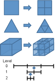
Figure 31: 自适应模式
43.3. 指示器对象
Indicator 报告每个单元的“误差”量,内置的 Indicators 包括:
GradientJumpIndicator: 变量梯度在单元边缘的跳跃。一个很好的“曲率”指示器,在各种问题上都表现良好。 FluxJumpIndicator: 与 GradientJump 类似,不同之处在于可以提供一个标量系数(例如导热系数)来产生一个物理的“通量”量。 LaplacianJumpIndicator: 变量二阶导数的跳跃。仅对 C 1 C 1
形函数有用。 AnalyticIndicator: 计算有限元解与用户提供的代表问题解析解的 Function 之间的差异。
43.4. 标记器对象
在 Indicator 计算完每个单元的误差后,必须使用 Marker 对象来决定是细化还是粗化单元。
ErrorFractionMarker: 根据它们对总误差的贡献来选择单元。 ErrorToleranceMaker: 如果误差大于指定值则细化,如果小于则粗化。 ValueThresholdMarker: 如果变量值大于特定值则细化,如果小于则粗化。 BoxMarker: 在给定框的内部或外部进行细化或粗化。 ComboMarker: 组合上述几个 Marker。
43.5. 输入语法
[Adaptivity]
initial_steps = 2
cycles_per_step = 2
marker = marker
initial_marker = marker
max_h_level = 2
[Indicators]
[indicator]
type = GradientJumpIndicator
variable = u
[]
[]
[Markers]
[marker]
type = ErrorFractionMarker
indicator = indicator
coarsen = 0.1
refine = 0.7
[]
[]
[]
44. 第 7 步:网格自适应
44.1. (续)
44.2. 第 7a 步:粗糙解
@@ -1,112 +1,112 @@
[Mesh]
[gmg]
type = GeneratedMeshGenerator
dim = 2

nx = 200
ny = 10
nx = 30
ny = 3
xmax = 0.304 # Length of test chamber
ymax = 0.0257 # Test chamber radius
[]
coord_type = RZ
rz_coord_axis = X
[]
[Variables]
[pressure]
[]
[temperature]

initial_condition = 300 # Start at room temperature
initial_condition = 300
[]
[]
[Kernels]
[darcy_pressure]
type = DarcyPressure
variable = pressure
[]
[heat_conduction]

type = ADHeatConduction
variable = temperature
type = ADHeatConduction
variable = temperature
[]
[heat_conduction_time_derivative]
type = ADHeatConductionTimeDerivative
variable = temperature
type = ADHeatConductionTimeDerivative
variable = temperature
[]
[heat_convection]
type = DarcyAdvection
variable = temperature
pressure = pressure
[]
[]
[BCs]
[inlet_temperature]

type = FunctionDirichletBC
variable = temperature
boundary = left
function = 'if(t<0,350+50*t,350)'
type = FunctionDirichletBC
variable = temperature
boundary = left
function = 'if(t<0,350+50*t,350)'
[]
[outlet_temperature]
type = HeatConductionOutflow
variable = temperature
boundary = right
[]
[inlet]
type = DirichletBC
variable = pressure
boundary = left
value = 4000 # (Pa) From Figure 2 from paper. First data point for 1mm spheres.
type = DirichletBC
variable = pressure
boundary = left
value = 4000
[]
[outlet]
type = DirichletBC
variable = pressure
boundary = right
value = 0 # (Pa) Gives the correct pressure drop from Figure 2 for 1mm spheres
type = DirichletBC
variable = pressure
boundary = right
value = 0
[]
[]
[Materials/column]
type = PackedColumn
temperature = temperature
radius = 1
[]

[AuxVariables/velocity]
order = CONSTANT
family = MONOMIAL_VEC
[]

[AuxKernels/velocity]
type = DarcyVelocity
variable = velocity
execute_on = timestep_end
pressure = pressure
[]

[Problem]
type = FEProblem
[]

[Executioner]
type = Transient
end_time = 100
dt = 0.25
start_time = -1

solve_type = NEWTON
petsc_options_iname = '-pc_type -pc_hypre_type'
petsc_options_value = 'hypre boomeramg'

automatic_scaling = true
steady_state_tolerance = 1e-5
steady_state_detection = true

[TimeStepper]
type = FunctionDT
function = 'if(t<0,0.1,0.25)'
[]
[]

[Outputs]

exodus = true
exodus = true
[]
44.3. 第 7a 步:运行
cd ~/projects/moose/tutorials/darcy_thermo_mech/step07_adaptivity
make -j 12 # 使用您系统的处理器数量
cd problems
../darcy_thermo_mech-opt -i step7a_coarse.i
44.4. 第 7b 步:精细解
@@ -1,112 +1,113 @@
[Mesh]
[gmg]
type = GeneratedMeshGenerator
dim = 2
nx = 30
ny = 3
xmax = 0.304 # Length of test chamber
ymax = 0.0257 # Test chamber radius
[]
coord_type = RZ
rz_coord_axis = X

uniform_refine = 3
[]
[Variables]
[pressure]
[]
[temperature]

initial_condition = 300 # Start at room temperature
initial_condition = 300
[]
[]
[Kernels]
[darcy_pressure]
type = DarcyPressure
variable = pressure
[]
[heat_conduction]

type = ADHeatConduction
variable = temperature
type = ADHeatConduction
variable = temperature
[]
[heat_conduction_time_derivative]
type = ADHeatConductionTimeDerivative
variable = temperature
type = ADHeatConductionTimeDerivative
variable = temperature
[]
[heat_convection]
type = DarcyAdvection
variable = temperature
pressure = pressure
[]
[]
[BCs]
[inlet_temperature]

type = FunctionDirichletBC
variable = temperature
boundary = left
function = 'if(t<0,350+50*t,350)'
type = FunctionDirichletBC
variable = temperature
boundary = left
function = 'if(t<0,350+50*t,350)'
[]
[outlet_temperature]
type = HeatConductionOutflow
variable = temperature
boundary = right
[]
[inlet]
type = DirichletBC
variable = pressure
boundary = left
value = 4000 # (Pa) From Figure 2 from paper. First data point for 1mm spheres.
type = DirichletBC
variable = pressure
boundary = left
value = 4000
[]
[outlet]
type = DirichletBC
variable = pressure
boundary = right
value = 0 # (Pa) Gives the correct pressure drop from Figure 2 for 1mm spheres
type = DirichletBC
variable = pressure
boundary = right
value = 0
[]
[]
[Materials/column]
type = PackedColumn
temperature = temperature
radius = 1
[]

[AuxVariables/velocity]
order = CONSTANT
family = MONOMIAL_VEC
[]

[AuxKernels/velocity]
type = DarcyVelocity
variable = velocity
execute_on = timestep_end
pressure = pressure
[]

[Problem]
type = FEProblem
[]

[Executioner]
type = Transient
end_time = 100
dt = 0.25
start_time = -1

solve_type = NEWTON
petsc_options_iname = '-pc_type -pc_hypre_type'
petsc_options_value = 'hypre boomeramg'

automatic_scaling = true
steady_state_tolerance = 1e-5
steady_state_detection = true

[TimeStepper]
type = FunctionDT
function = 'if(t<0,0.1,0.25)'
[]
[]

[Outputs]

exodus = true
exodus = true
[]
44.5. 第 7b 步:运行
cd ~/projects/moose/tutorials/darcy_thermo_mech/step07_adaptivity
make -j 12 # 使用您系统的处理器数量
cd problems
../darcy_thermo_mech-opt -i step7b_fine.i
44.6. 第 7c 步:自适应网格解
@@ -1,113 +1,129 @@
[Mesh]
[gmg]
type = GeneratedMeshGenerator
dim = 2
nx = 30
ny = 3
xmax = 0.304 # Length of test chamber
ymax = 0.0257 # Test chamber radius
[]
coord_type = RZ
rz_coord_axis = X

uniform_refine = 3
uniform_refine = 3 # This is now the max_h_level, not a uniform refinement
[]
[Variables]
[pressure]
[]
[temperature]

initial_condition = 300 # Start at room temperature
initial_condition = 300
[]
[]
[Kernels]
[darcy_pressure]
type = DarcyPressure
variable = pressure
[]
[heat_conduction]

type = ADHeatConduction
variable = temperature
type = ADHeatConduction
variable = temperature
[]
[heat_conduction_time_derivative]
type = ADHeatConductionTimeDerivative
variable = temperature
type = ADHeatConductionTimeDerivative
variable = temperature
[]
[heat_convection]
type = DarcyAdvection
variable = temperature
pressure = pressure
[]
[]
[BCs]
[inlet_temperature]

type = FunctionDirichletBC
variable = temperature
boundary = left
function = 'if(t<0,350+50*t,350)'
type = FunctionDirichletBC
variable = temperature
boundary = left
function = 'if(t<0,350+50*t,350)'
[]
[outlet_temperature]
type = HeatConductionOutflow
variable = temperature
boundary = right
[]
[inlet]
type = DirichletBC
variable = pressure
boundary = left
value = 4000 # (Pa) From Figure 2 from paper. First data point for 1mm spheres.
type = DirichletBC
variable = pressure
boundary = left
value = 4000
[]
[outlet]
type = DirichletBC
variable = pressure
boundary = right
value = 0 # (Pa) Gives the correct pressure drop from Figure 2 for 1mm spheres
type = DirichletBC
variable = pressure
boundary = right
value = 0
[]
[]
[Materials/column]
type = PackedColumn
temperature = temperature
radius = 1
[]

[AuxVariables/velocity]
order = CONSTANT
family = MONOMIAL_VEC
[]

[AuxKernels/velocity]
type = DarcyVelocity
variable = velocity
execute_on = timestep_end
pressure = pressure
[]

[Problem]
type = FEProblem
[]

[Executioner]
type = Transient
end_time = 100
dt = 0.25
start_time = -1

solve_type = NEWTON
petsc_options_iname = '-pc_type -pc_hypre_type'
petsc_options_value = 'hypre boomeramg'

automatic_scaling = true
steady_state_tolerance = 1e-5
steady_state_detection = true

[TimeStepper]
type = FunctionDT
function = 'if(t<0,0.1,0.25)'
[]
[]

[Outputs]

exodus = true
exodus = true
+[]
+[Adaptivity]

marker = error_frac
max_h_level = 3
[Indicators/temperature_jump]
type = GradientJumpIndicator
variable = temperature
scale_by_flux_faces = true
[]
[Markers/error_frac]
type = ErrorFractionMarker
coarsen = 0.15
indicator = temperature_jump
refine = 0.7
[]
[]
44.7. 第 7c 步:运行
cd ~/projects/moose/tutorials/darcy_thermo_mech/step07_adaptivity
make -j 12 # 使用您系统的处理器数量
cd problems
../darcy_thermo_mech-opt -i step7a_adapt.i
44.8. 第 7d 步:多个子域
@@ -1,129 +1,161 @@
[Mesh]
[gmg]
type = GeneratedMeshGenerator
dim = 2

nx = 30
ny = 3
nx = 40
ny = 4
xmax = 0.304 # Length of test chamber
ymax = 0.0257 # Test chamber radius
[]
[bottom]
type = SubdomainBoundingBoxGenerator
input = gmg
location = inside
bottom_left = '0 0 0'
top_right = '0.304 0.01285 0'
block_id = 1
[]
coord_type = RZ
rz_coord_axis = X
uniform_refine = 3
uniform_refine = 3 # This is now the max_h_level, not a uniform refinement
[]
[Variables]
[pressure]
[]
[temperature]

initial_condition = 300 # Start at room temperature
initial_condition = 300
[]
[]
[Kernels]
[darcy_pressure]
type = DarcyPressure
variable = pressure
[]
[heat_conduction]

type = ADHeatConduction
variable = temperature
type = ADHeatConduction
variable = temperature
[]
[heat_conduction_time_
Generated org
derivative]
-    type = ADHeatConductionTimeDerivative
-    variable = temperature
+    type = ADHeatConductionTimeDerivative
+    variable = temperature
   []
   [heat_convection]
     type = DarcyAdvection
     variable = temperature
     pressure = pressure
   []
 []

 [BCs]
   [inlet_temperature]
-    type = FunctionDirichletBC
-    variable = temperature
-    boundary = left
-    function = 'if(t<0,350+50*t,350)'
+    type = FunctionDirichletBC
+    variable = temperature
+    boundary = left
+    function = 'if(t<0,350+50*t,350)'
   []
   [outlet_temperature]
     type = HeatConductionOutflow
     variable = temperature
     boundary = right
   []
   [inlet]
-    type = DirichletBC
-    variable = pressure
-    boundary = left
-    value = 4000 # (Pa) From Figure 2 from paper.  First data point for 1mm spheres.
+    type = DirichletBC
+    variable = pressure
+    boundary = left
+    value = 4000
   []
   [outlet]
-    type = DirichletBC
-    variable = pressure
-    boundary = right
-    value = 0 # (Pa) Gives the correct pressure drop from Figure 2 for 1mm spheres
+    type = DirichletBC
+    variable = pressure
+    boundary = right
+    value = 0
   []
 []

-[Materials/column]
--  type = PackedColumn
--  temperature = temperature
--  radius = 1
+[Materials]
+  viscosity_file = data/water_viscosity.csv
+  density_file = data/water_density.csv
+  thermal_conductivity_file = data/water_thermal_conductivity.csv
+  specific_heat_file = data/water_specific_heat.csv
+
+  [column_bottom]
+    type = PackedColumn
+    block = 1
+    radius = 1.15
+    temperature = temperature
+    fluid_viscosity_file = ${viscosity_file}
+    fluid_density_file = ${density_file}
+    fluid_thermal_conductivity_file = ${thermal_conductivity_file}
+    fluid_specific_heat_file = ${specific_heat_file}
+  []
+  [column_top]
+    type = PackedColumn
+    block = 0
+    radius = 1
+    temperature = temperature
+    porosity = '0.25952 + 0.7*x/0.304'
+    fluid_viscosity_file = ${viscosity_file}
+    fluid_density_file = ${density_file}
+    fluid_thermal_conductivity_file = ${thermal_conductivity_file}
+    fluid_specific_heat_file = ${specific_heat_file}
+  []
 []

 [AuxVariables/velocity]
   order = CONSTANT
   family = MONOMIAL_VEC
 []

 [AuxKernels/velocity]
   type = DarcyVelocity
   variable = velocity
   execute_on = timestep_end
   pressure = pressure
 []

 [Problem]
   type = FEProblem
 []

 [Executioner]
   type = Transient
   end_time = 100
   dt = 0.25
   start_time = -1

   solve_type = NEWTON
   petsc_options_iname = '-pc_type -pc_hypre_type'
   petsc_options_value = 'hypre boomeramg'

   automatic_scaling = true
   steady_state_tolerance = 1e-5
   steady_state_detection = true

   [TimeStepper]
     type = FunctionDT
     function = 'if(t<0,0.1,0.25)'
   []
 []

-[Outputs]
--  exodus = true
+[Outputs/out]
+  type = Exodus
+  output_material_properties = true
 []

 [Adaptivity]
   marker = error_frac
   max_h_level = 3
   [Indicators/temperature_jump]
-    type = GradientJumpIndicator
-    variable = temperature
-    scale_by_flux_faces = true
+    type = GradientJumpIndicator
+    variable = temperature
+    scale_by_flux_faces = true
   []
   [Markers/error_frac]
-    type = ErrorFractionMarker
--    coarsen = 0.15
--    indicator = temperature_jump
--    refine = 0.7
+    type = ErrorFractionMarker
+    coarsen = 0.025
+    indicator = temperature_jump
+    refine = 0.9
   []
 []
45. 第 8 步:后处理器
基于仿真数据的聚合值对于理解仿真以及定义耦合方程之间的耦合值非常有用。
有两个主要系统用于聚合数据:`Postprocessors` 和 `VectorPostprocessors`。
所有 MOOSE Postprocessors 都基于 UserObject 系统,因此我们将从那里开始介绍。
46. UserObject 系统
一个用于在 MOOSE 对象之间定义任意接口的系统。
`UserObject` 系统向其他 MOOSE 对象提供数据和计算结果。
- `Postprocessors` 是计算单个标量值的 UserObjects。
- `VectorPostprocessors` 是计算数据向量的 UserObjects。
- `UserObjects` 定义自己的接口,其他 MOOSE 对象可以调用该接口来检索数据。
46.1. 执行
`UserObjects` 通过输入文件中的 `executeon` 选项在指定的“时间”计算:
- `executeon = 'initial timestepend'`
- `executeon = linear`
- `executeon = nonlinear`
- `executeon = 'timestepbegin final failed'`
它们可以限制在特定的块、边集和节点集上。
46.2. UserObject 类型
`UserObject` 有多种类型:
- `ElementUserObject`: 在单元上执行
- `NodalUserObject`: 在节点上执行
- `SideUserObject`: 在边界上的边上执行
- `InternalSideUserObject`: 在内部边上执行
- `InterfaceUserObject`: 在界面上的边上执行
- `DomainUserObject`: 在单元、内部和外部边上执行
- `GeneralUserObject`: 执行一次
46.3. UserObject 解剖
- `virtual void initialize();`: 在开始 `UserObject` 计算之前调用一次。
- `virtual void execute();`: 在每个几何实体(单元、节点等)上调用一次,或者对于 `GeneralUserObject` 每次计算调用一次。
- `virtual void threadJoin(const UserObject & uo);`: 在线程执行期间,此函数用于“连接”在不同线程上生成的计算。
- 将 `uo` 转换为特定 `UserObject` 类型的 `const` 引用,然后提取数据并将其聚合到“this”对象中的数据。
- `GeneralUserObject` 不需要此函数,因为它*不是*线程化的。
- `virtual void finalize();`: 所有计算完成后调用的最后一个函数。
- 从 `execute()` 中执行的所有计算中获取数据,并执行一个操作以获得最终值。
- 在必要时执行并行通信,以确保所有处理器计算出相同的值。
46.4. 用户定义的接口
`UserObject` 通过定义 `const` 函数来定义自己的接口。
例如,如果一个 `UserObject` 正在计算网格中每个块上变量的平均值,它可能会提供一个像这样的函数:
Real averageValue(SubdomainID block) const;
需要此 `UserObject` 的另一个 `MooseObject` 将调用 `averageValue()` 来获取计算结果。
46.5. 使用 UserObject
任何 MOOSE 对象都可以以类似于检索 `Function` 的方式检索 `UserObject`。
通常,从输入文件中获取 `UserObject` 的名称是一个好主意:
InputParameters
BlockAverageDiffusionMaterial::validParams()
{
  InputParameters params = Material::validParams();
  params.addRequiredParam<UserObjectName>("block_average_userobject", "Computes the ...");
  return params;
}
`UserObject` 以 `UserObject` 类型的 `const` 引用形式出现。因此,在您的对象中:
const BlockAverageValue & _block_average_value;
引用是通过调用模板化的 `getUserObject()` 方法在对象的初始化列表中设置的:
BlockAverageDiffusionMaterial::BlockAverageDiffusionMaterial(const InputParameters & parameters) :
    Material(parameters),
    _block_average_value(getUserObject<BlockAverageValue>("block_average_userobject"))
{}
通过调用 `UserObject` 定义的一些接口函数来使用引用:
_diffusivity[_qp] = 0.5 * _block_average_value.averageValue(_current_elem->subdomain_id());
47. 后处理器系统
一个用于基于解变量计算“归约”或“聚合”计算,从而得到*单个*标量值的系统。
47.1. 后处理器类型
在 `::compute…` 例程中定义的操作根据后处理器类型应用于不同位置。
- `ElementPostprocessor`: 对每个单元进行操作
- `NodalPostprocessor`: 对每个节点进行操作
- `SidePostprocessor`: 对边界上的每个单元侧面进行操作
- `InternalSidePostprocessor`: 对内部单元侧面进行操作
- `InterfacePostprocessor`: 对子域界面上的每个单元侧面进行操作
- `GeneralPostprocessor`: 每次执行操作一次
47.2. 后处理器剖析
`Postprocessor` 是一个 `UserObject`,因此可以定义 `initialize`、`execute`、`threadJoin` 和 `finalize` 方法。
- `initialize()`: 每次执行前调用一次。用于重置累积量。
- `execute()`: 定义了在每个单元/侧面/节点/网格(取决于类型)上执行的操作。求积积分通常在这里定义,用户通常不需要定义这个。
- `Real getValue()`: 在 MOOSE 内部调用以检索最终的标量值,此函数返回的值被所有其他使用该后处理器的对象引用。
大多数 `Postprocessor` 基类已经为您定义了这些例程!
47.3. 聚合例程
如果创建的 `Postprocessor` 具有自定义数据,则必须确保在(MPI 和基于线程的)并行仿真中正确通信该值。
对于 MPI,存在几种实用方法来执行常见的聚合操作:
- `gatherSum(scalar)`: 在所有处理器上求和。
- `gatherMin(scalar)`: 从所有处理器中取最小值。
- `gatherMax(scalar)`: 从所有处理器中取最大值。
47.4. 内置后处理器类型
MOOSE 包含了大量内置的 `Postprocessors`: `ElementAverageValue`, `SideAverageValue`, `ElementL2Error`, `ElementH1Error` 等等。
默认情况下,`Postprocessors` 将输出到屏幕上的格式化表格,并可选地使用 `[Outputs]` 块存储在 CSV 文件中。
[Output]
  csv = true
[]
47.5. 使用后处理器
通过创建对 `PostprocessorValue` 的 `const` 引用并在对象构造函数的初始化列表中初始化该引用,可以在对象中使用后处理器值。
在头文件中,我们声明一个引用,
const PostprocessorValue & _pps_value;
在源文件中,我们检索对后处理器值的引用,
_pps_value(getPostprocessorValue("postprocessor")),
47.6. 默认后处理器值
可以为 `Postprocessors` 设置默认值,以允许对象在不创建或指定 `Postprocessor` 对象的情况下运行。
params.addParam<PostprocessorName>("postprocessor", 1.2345, "Doc String");
此外,可以在输入文件中提供一个值来代替 `Postprocessor` 名称。
48. 向量后处理器系统
一个用于基于解变量进行“归约”或“聚合”计算,从而得到一个或多个值向量的系统。
48.1. 向量后处理器类型
在 `::compute…` 例程中定义的操作根据 `VectorPostprocessor` 类型应用于不同位置。
- `ElementVectorPostprocessor`: 对每个单元进行操作
- `NodalVectorPostprocessor`: 对每个节点进行操作
- `SideVectorPostprocessor`: 对边界上的每个单元侧面进行操作
- `InternalSideVectorPostprocessor`: 对内部单元侧面进行操作
- `GeneralVectorPostprocessor`: 每次执行操作一次
48.2. 向量后处理器剖析
`VectorPostprocessor` 是一个 `UserObject`,因此 `initialize`、`execute`、`threadJoin` 和 `finalize` 方法用于实现聚合操作。
- `virtual VectorPostprocessorValue & getVector (const std::string &vectorname)`: 在 MOOSE 内部调用以检索给定名称的最终向量值,此函数返回的值被所有其他使用该向量后处理器的对象引用。
`VectorPostprocessor` 对象的操作有点像 `Material` 对象,每个向量都被声明,然后在 `initialize`、`execute`、`threadJoin` 和 `finalize` 方法中用所需的数据更新向量。
创建一个成员变量,作为对向量数据的引用。
VectorPostprocessorValue & _pid;
使用 `declareVector` 方法和名称初始化引用。
_pid(declareVector("pid")),
48.3. 内置向量后处理器类型
MOOSE 包含了大量内置的 `VectorPostprocessors`: `NodalValueSampler`, `LineValueSampler`, `PointValueSampler` 等等。
`VectorPostprocessors` 的输出可以通过 `[Outputs]` 块选择性地启用。将为每个向量和时间步创建一个 CSV 文件。
[Output]
  csv = true
[]
48.4. 使用向量后处理器
通过创建对 `VectorPostprocessorValue` 的 `const` 引用并在初始化列表中初始化该引用,可以在对象中使用后处理器值。
const VectorPostprocessorValue & _x_values;
_x_values(getVectorPostprocessorValue("vectorpostprocessor", _x_name)),
49. 第 8 步:后处理器
49.1. (续)
49.2. 第 8 步:输入文件
 @@ -1,112 +1,137 @@
 [Mesh]
   [gmg]
     type = GeneratedMeshGenerator
     dim = 2
-    nx = 200
-    ny = 10
+    nx = 30
+    ny = 3
     xmax = 0.304 # Length of test chamber
     ymax = 0.0257 # Test chamber radius
   []
   coord_type = RZ
   rz_coord_axis = X
+  uniform_refine = 2
 []

 [Variables]
   [pressure]
   []
   [temperature]
-    initial_condition = 300 # Start at room temperature
+    initial_condition = 300
   []
 []

 [Kernels]
   [darcy_pressure]
     type = DarcyPressure
     variable = pressure
   []
   [heat_conduction]
-    type = ADHeatConduction
-    variable = temperature
+    type = ADHeatConduction
+    variable = temperature
   []
   [heat_conduction_time_derivative]
-    type = ADHeatConductionTimeDerivative
-    variable = temperature
+    type = ADHeatConductionTimeDerivative
+    variable = temperature
   []
   [heat_convection]
     type = DarcyAdvection
     variable = temperature
     pressure = pressure
   []
 []

 [BCs]
   [inlet_temperature]
-    type = FunctionDirichletBC
-    variable = temperature
-    boundary = left
-    function = 'if(t<0,350+50*t,350)'
+    type = FunctionDirichletBC
+    variable = temperature
+    boundary = left
+    function = 'if(t<0,350+50*t,350)'
   []
   [outlet_temperature]
     type = HeatConductionOutflow
     variable = temperature
     boundary = right
   []
   [inlet]
-    type = DirichletBC
-    variable = pressure
-    boundary = left
-    value = 4000 # (Pa) From Figure 2 from paper.  First data point for 1mm spheres.
+    type = DirichletBC
+    variable = pressure
+    boundary = left
+    value = 4000
   []
   [outlet]
-    type = DirichletBC
-    variable = pressure
-    boundary = right
-    value = 0 # (Pa) Gives the correct pressure drop from Figure 2 for 1mm spheres
+    type = DirichletBC
+    variable = pressure
+    boundary = right
+    value = 0
   []
 []

 [Materials/column]
   type = PackedColumn
   temperature = temperature
   radius = 1
+  porosity = '0.25952 + 0.7*y/0.0257'
+[]
+
+[Postprocessors]
+  [average_temperature]
+    type = ElementAverageValue
+    variable = temperature
+  []
+  [outlet_heat_flux]
+    type = ADSideDiffusiveFluxIntegral
+    variable = temperature
+    boundary = right
+    diffusivity = thermal_conductivity
+  []
+[]
+
+[VectorPostprocessors/temperature_sample]
+  type = LineValueSampler
+  num_points = 500
+  start_point = '0.1 0      0'
+  end_point =   '0.1 0.0257 0'
+  variable = temperature
+  sort_by = y
 []

 [AuxVariables/velocity]
   order = CONSTANT
   family = MONOMIAL_VEC
 []

 [AuxKernels/velocity]
   type = DarcyVelocity
   variable = velocity
   execute_on = timestep_end
   pressure = pressure
 []

 [Problem]
   type = FEProblem
 []

 [Executioner]
   type = Transient
   end_time = 100
   dt = 0.25
   start_time = -1

   solve_type = NEWTON
   petsc_options_iname = '-pc_type -pc_hypre_type'
   petsc_options_value = 'hypre boomeramg'

   automatic_scaling = true
   steady_state_tolerance = 1e-5
   steady_state_detection = true

   [TimeStepper]
     type = FunctionDT
     function = 'if(t<0,0.1,0.25)'
   []
 []

 [Outputs]
-  exodus = true
+  exodus = true
+  csv = true
 []
49.3. 第 8 步:运行
cd ~/projects/moose/tutorials/darcy_thermo_mech/step08_postprocessors
make -j 12 # 使用您系统的处理器数量
cd problems
../darcy_thermo_mech-opt -i step8.i
50. 第 9 步:力学
50.1. 力学
计算如果管子只允许沿轴向 (y) 方向膨胀时的弹性和热应变。
\[\begin{aligned} \nabla \cdot \boldsymbol{\sigma} + \mathbf{b} &= \mathbf{0} \\ \boldsymbol{\sigma} &= \mathbf{C} : (\boldsymbol{\epsilon} - \boldsymbol{\epsilon}_{thermal}) + \boldsymbol{\sigma}_{eigen} \\ \boldsymbol{\epsilon} &= \frac{1}{2} (\nabla\mathbf{u} + (\nabla\mathbf{u})^T) \\ \mathbf{u} &= \bar{\mathbf{u}} \quad \text{on } \Gamma_D \\ \boldsymbol{\sigma} \cdot \mathbf{n} &= \bar{\mathbf{t}} \quad \text{on } \Gamma_N \end{aligned}\]
其中 \(\boldsymbol{\sigma}\) 是柯西应力张量,\(\boldsymbol{\sigma}_{eigen}\) 是额外的应力源(如孔隙压力),\(\mathbf{u}\) 是位移向量,\(\mathbf{b}\) 是体力,\(\mathbf{n}\) 是边界的单位法线,\(\bar{\mathbf{u}}\) 是边界上规定的位移,\(\bar{\mathbf{t}}\) 是边界上规定的牵引力。
51. 模块
51.1. 化学反应
提供一套用于计算多孔介质中多组分水溶液反应输运的工具,最初是作为 MOOSE 应用程序 RAT (Guo et al., 2013) 开发的。
51.2. 接触
提供必要的工具,使用算法在网格中的表面之间强制约束,以防止穿透和产生接触力来模拟机械接触。
51.3. 接触:摩擦熨烫问题
51.4. 电磁学
电磁学模块提供组件和模型,以使用 MOOSE 模拟电磁波问题,并促进电磁仿真与其他物理域的耦合。麦克斯韦方程组在 1-D 和 2-D 中使用亥姆霍兹波动方程公式求解复场。还为不完美的电接口提供了静电接触。
51.5. 外部 PETSc 求解器
提供对要与基于 moose 的应用程序耦合的独立原生 PETSc 应用程序的支持。它也是与外部应用程序耦合的通用示例。
51.6. 流体属性
流体属性模块为流体属性(如密度、粘度、焓等)以及相对于主要变量的导数提供了一致的接口。该一致接口允许在输入文件中通过简单地交换流体属性 UserObject 的名称以即插即用的方式使用不同的流体。
51.7. 流固耦合
提供用于解决流体和结构问题的工具,其中它们的行为是相互依赖的。目前能够使用流体的声学公式模拟流固耦合行为。
Figure 32: 晃动 GIF
51.8. 函数展开工具
一个用于连续、网格无关、高保真、减少数据的 MultiApp 耦合的 MOOSE 模块。
函数展开 (FXs) 是一种将信息表示为函数级数矩的方法 (Flusser et al., 2016)。这与循环数据的傅立叶级数表示有关。通过对函数级数中的每一项进行数值积分来生成矩,以表示感兴趣的场。然后,这些矩可用于在单独的应用程序中重构场 (Wendt et al., 2018; Wendt and Kerby, 2017; Kerby et al., 2017)。
51.9. 地球化学
解决地球化学模型。能力包括:
- 平衡水溶液系统
- 氧化还原非平衡
- 吸附和表面络合
- 动力学
- 以上所有与流体和热传输相结合
它旨在轻松与多孔流模块接口,以便可以研究复杂的反应输运场景。
51.10. 热传递
用于求解瞬态热传导方程的基本实用程序:
\[\rho c_p \frac{\partial T}{\partial t} - \nabla \cdot (k \nabla T) = Q_{source}\]
还包含广义热传递(对流、辐射…)的能力。
51.11. 水平集
水平集模块提供了解决水平集方程的基本功能,该方程就是多维平流方程:
\[\frac{\partial \phi}{\partial t} + \mathbf{v} \cdot \nabla \phi = 0\]
51.12. 纳维-斯托克斯
一个用于实现仿真工具的库,该工具使用连续伽辽金有限元 (CGFE) 或有限体积 (FV) 方法求解多维纳维-斯托克斯方程。纳维-斯托克斯方程可以用以下方式求解:
- 不可压缩公式 (CGFE & FV)
- 弱可压缩公式 (FV)
- 全可压缩公式 (FV)
提供零维湍流模型,并且很快将添加粗糙正则化 k-epsilon。
51.13. 纳维-斯托克斯
盖驱动腔内 Re=417(左)和 Re=833(右)的流动。
Figure 33: NS Re=417
Figure 34: NS Re=833
51.14. 优化
MOOSE 优化模块提供了在 MOOSE 中解决逆优化问题的功能。它基于使用 PETSc TAO 优化求解器的 PDE 约束优化。
Figure 35: 优化循环图
\(\min_{p} J(u, p)\) subject to \(R(u, p)=0\) and \(g(u,p) \le 0\)
51.15. 相场
MOOSE 相场模块是一个用于简化采用相场模型的仿真工具实现的库。
51.16. 多孔流
PorousFlow 模块是一个用于多孔介质中流体和热流动的物理库。它的公式极其通用,因此能够使用任意一组主变量解决具有任意数量相(气体、液体等)和流体组分(每个流体相中存在的物种)的问题。
51.17. 射线追踪
提供在有限元网格中追踪射线的功能。显著特点包括:
- 对沿射线的残差和雅可比的贡献
- 射线与内部和外部边界的相互作用
- 支持存储和操作每条射线独有的数据
- 支持射线与场变量的相互作用
- 高度并行化:在 20k MPI 级别上测试过
51.18. 射线追踪:手电筒光源

Figure 36: 手电筒源 u

Figure 37: 手电筒源射线
51.19. 重构不连续伽辽金 (rDG)
MOOSE rDG 模块是一个用于实现仿真工具的库,该工具使用所谓的重构不连续伽辽金 (rDG) 方法来解决对流主导的问题。此模块中实现的特定 rDG 方法是 rDG(P0P1),它等效于二阶单元中心有限体积法 (FVM)。
51.20. 反应堆
向 MOOSE 添加了高级网格划分功能,以便用户可以创建与反应堆堆芯结构相关的复杂几何网格。这包括:
- 为组件创建和修改六边形网格组件
- 将组件拼接在一起形成堆芯网格
- 为组件和堆芯创建外围区域
- 为燃料棒和组件区域添加 ID
- 启用旋转控制鼓的动态和静态仿真。
51.21. 反应堆:微型反应堆网格划分
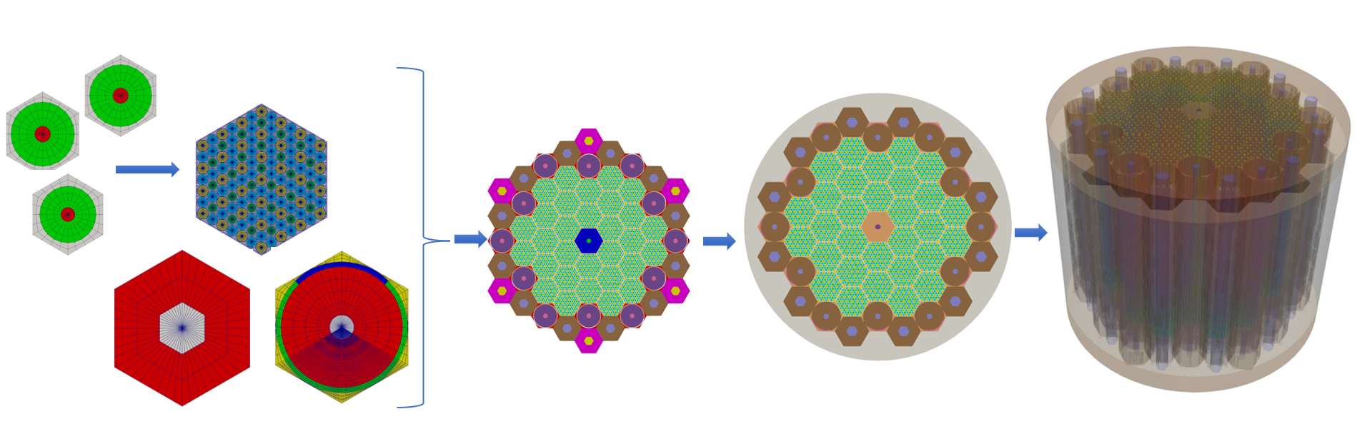
Figure 38: 反应堆微型反应堆
51.22. 随机工具
Figure 39: 随机工具
51.23. 固体力学
固体力学模块是一个用于解决连续介质力学问题的仿真工具库。该模块可用于模拟线性和有限应变力学,包括弹性和 Cosserat 弹性、塑性和微观力学塑性、蠕变以及由于开裂和性能退化引起的损伤。
51.24. 热工水力
热工水力模块是一个可用于构建热工水力仿真的组件库。基本功能包括一个单相、可变面积、无粘性、可压缩流动模型,带有不可凝结蒸汽混合物,二维和三维热传导,一个控制逻辑系统,以及可插拔的闭合系统和模型。
51.25. 扩展有限元法 (XFEM)
一个基于 MOOSE 的扩展有限元法实现,这是一种专门设计用于处理不连续性的数值方法。
52. 网格系统(续)
52.1. 复制网格
在并行运行时,默认操作模式是使用复制网格,它为每个处理器创建网格的完整副本。
[Mesh]
  parallel_type = replicated
[]
52.2. 分布式网格
在并行运行时将类型更改为 `distributed`,这样只有处理器拥有的网格部分存储在该处理器上。
[Mesh]
  parallel_type = distributed
[]
如果网格太大而无法在单个处理器上读入,可以在仿真之前将其拆分。(可以使用 `partmesh.py`)
52.3. 位移网格
计算可以在初始网格配置中进行,或者在请求时,在“位移”配置中进行。
要在网格块中启用位移,请为每个空间维度提供位移变量名称的向量。
[Mesh]
  [gen]
    type = GeneratedMeshGenerator
    dim = 2
    xmin = 0
    ymin = 0
    xmax = 0.2
    ymax = 0.5
    nx = 5
    ny = 15
    elem_type = QUAD4
  []
  displacements = 'disp_x disp_y'
[]
对象可以在 `validParams` 函数中强制使用位移网格。
params.set<bool>("use_displaced_mesh") = true;
53. 第 9 步:力学
53.1. (续)
53.2. PackedColumn.h
 @@ -1,95 +1,108 @@

 #pragma once

 #include "Material.h"

 // A helper class from MOOSE that linear interpolates x,y data
 #include "LinearInterpolation.h"

 /**
  * Material objects inherit from Material and override computeQpProperties.
  *
  * Their job is to declare properties for use by other objects in the
  * calculation such as Kernels and BoundaryConditions.
  */
 class PackedColumn : public Material
 {
 public:
   static InputParameters validParams();

   PackedColumn(const InputParameters & parameters);

 protected:
   /// Necessary override. This is where the values of the properties are computed.
   virtual void computeQpProperties() override;

   /**
    * Helper function for reading CSV data for use in an interpolator object.
    */
   bool initInputData(const std::string & param_name, ADLinearInterpolation & interp);

   /// The radius of the spheres in the column
   const Function & _input_radius;

   /// The input porosity
   const Function & _input_porosity;

   /// Temperature
   const ADVariableValue & _temperature;

   /// Compute permeability based on the radius (mm)
   LinearInterpolation _permeability_interpolation;

   /// Fluid viscosity
   bool _use_fluid_mu_interp;
   const Real & _fluid_mu;
   ADLinearInterpolation _fluid_mu_interpolation;

   /// Fluid thermal conductivity
   bool _use_fluid_k_interp = false;
   const Real & _fluid_k;
   ADLinearInterpolation _fluid_k_interpolation;

   /// Fluid density
   bool _use_fluid_rho_interp = false;
   const Real & _fluid_rho;
   ADLinearInterpolation _fluid_rho_interpolation;

   /// Fluid specific heat
   bool _use_fluid_cp_interp;
   const Real & _fluid_cp;
   ADLinearInterpolation _fluid_cp_interpolation;

+  /// Fluid thermal expansion coefficient
+  bool _use_fluid_cte_interp;
+  const Real & _fluid_cte;
+  ADLinearInterpolation _fluid_cte_interpolation;
+
   /// Solid thermal conductivity
   bool _use_solid_k_interp = false;
   const Real & _solid_k;
   ADLinearInterpolation _solid_k_interpolation;

   /// Solid density
   bool _use_solid_rho_interp = false;
   const Real & _solid_rho;
   ADLinearInterpolation _solid_rho_interpolation;

   /// Solid specific heat
   bool _use_solid_cp_interp;
   const Real & _solid_cp;
   ADLinearInterpolation _solid_cp_interpolation;
+
+  /// Solid thermal expansion coefficient
+  bool _use_solid_cte_interp;
+  const Real & _solid_cte;
+  ADLinearInterpolation _solid_cte_interpolation;

   /// The permeability (K)
   ADMaterialProperty<Real> & _permeability;

   /// The viscosity of the fluid (mu)
   ADMaterialProperty<Real> & _viscosity;

   /// The porosity (eps)
   ADMaterialProperty<Real> & _porosity;

   /// The bulk thermal conductivity
   ADMaterialProperty<Real> & _thermal_conductivity;

   /// The bulk heat capacity
   ADMaterialProperty<Real> & _specific_heat;

   /// The bulk density
   ADMaterialProperty<Real> & _density;
+
+  /// The bulk thermal expansion coefficient
+  ADMaterialProperty<Real> & _thermal_expansion;
 };
53.3. PackedColumn.C
 @@ -1,177 +1,201 @@

 #include "PackedColumn.h"
 #include "Function.h"
 #include "DelimitedFileReader.h"

 registerMooseObject("DarcyThermoMechApp", PackedColumn);

 InputParameters
 PackedColumn::validParams()
 {
   InputParameters params = Material::validParams();
   params.addRequiredCoupledVar("temperature", "The temperature (C) of the fluid.");

   // Parameter for radius of the spheres used to interpolate permeability.
   params.addParam<FunctionName>("radius",
                                 "1.0",
                                 "The radius of the steel spheres (mm) that are packed in the "
                                 "column for computing permeability.");

   // http://en.wikipedia.org/wiki/Close-packing_of_equal_spheres
   params.addParam<FunctionName>(
       "porosity", 0.25952, "Porosity of porous media, default is for closed packed spheres.");

   // Fluid properties
   params.addParam<Real>(
       "fluid_viscosity", 1.002e-3, "Fluid viscosity (Pa s); default is for water at 20C).");
   params.addParam<FileName>(
       "fluid_viscosity_file",
       "The name of a file containing the fluid viscosity (Pa-s) as a function of temperature "
       "(C); if provided the constant value is ignored.");

   params.addParam<Real>("fluid_thermal_conductivity",
                         0.59803,
                         "Fluid thermal conductivity (W/(mK); default is for water at 20C).");
   params.addParam<FileName>(
       "fluid_thermal_conductivity_file",
       "The name of a file containing fluid thermal conductivity (W/(mK)) as a function of "
       "temperature (C); if provided the constant value is ignored.");

   params.addParam<Real>(
       "fluid_density", 998.21, "Fluid density (kg/m^3); default is for water at 20C).");
   params.addParam<FileName>("fluid_density_file",
                             "The name of a file containing fluid density (kg/m^3) as a function "
                             "of temperature (C); if provided the constant value is ignored.");

   params.addParam<Real>(
       "fluid_specific_heat", 4157.0, "Fluid specific heat (J/(kgK); default is for water at 20C).");
   params.addParam<FileName>(
       "fluid_specific_heat_file",
       "The name of a file containing fluid specific heat (J/(kgK) as a function of temperature "
       "(C); if provided the constant value is ignored.");
+
+  params.addParam<Real>("fluid_thermal_expansion",
+                        2.07e-4,
+                        "Fluid thermal expansion coefficient (1/K); default is for water at 20C).");
+  params.addParam<FileName>("fluid_thermal_expansion_file",
+                            "The name of a file containing fluid thermal expansion coefficient "
+                            "(1/K) as a function of temperature "
+                            "(C); if provided the constant value is ignored.");

   // Solid properties
   // https://en.wikipedia.org/wiki/Stainless_steel#Properties
   params.addParam<Real>("solid_thermal_conductivity",
                         15.0,
                         "Solid thermal conductivity (W/(mK); default is for AISI/ASTIM 304 "
                         "stainless steel at 20C).");
   params.addParam<FileName>(
       "solid_thermal_conductivity_file",
       "The name of a file containing solid thermal conductivity (W/(mK)) as a function of "
       "temperature (C); if provided the constant value is ignored.");

   params.addParam<Real>(
       "solid_density",
       7900,
       "Solid density (kg/m^3); default is for AISI/ASTIM 304 stainless steel at 20C).");
   params.addParam<FileName>("solid_density_file",
                             "The name of a file containing solid density (kg/m^3) as a function "
                             "of temperature (C); if provided the constant value is ignored.");

   params.addParam<Real>(
       "solid_specific_heat",
       500,
       "Solid specific heat (J/(kgK); default is for AISI/ASTIM 304 stainless steel at 20C).");
   params.addParam<FileName>(
       "solid_specific_heat_file",
       "The name of a file containing solid specific heat (J/(kgK) as a function of temperature "
       "(C); if provided the constant value is ignored.");
+
+  params.addParam<Real>("solid_thermal_expansion",
+                        17.3e-6,
+                        "Solid thermal expansion coefficient (1/K); default is for water at 20C).");
+  params.addParam<FileName>("solid_thermal_expansion_file",
+                            "The name of a file containing solid thermal expansion coefficient "
+                            "(1/K) as a function of temperature "
+                            "(C); if provided the constant value is ignored.");
   return params;
 }

 PackedColumn::PackedColumn(const InputParameters & parameters)
   : Material(parameters),

     // Get the parameters from the input file
     _input_radius(getFunction("radius")),
     _input_porosity(getFunction("porosity")),
     _temperature(adCoupledValue("temperature")),

     // Fluid
     _fluid_mu(getParam<Real>("fluid_viscosity")),
     _fluid_k(getParam<Real>("fluid_thermal_conductivity")),
     _fluid_rho(getParam<Real>("fluid_density")),
     _fluid_cp(getParam<Real>("fluid_specific_heat")),
+    _fluid_cte(getParam<Real>("fluid_thermal_expansion")),

     // Solid
     _solid_k(getParam<Real>("solid_thermal_conductivity")),
     _solid_rho(getParam<Real>("solid_density")),
     _solid_cp(getParam<Real>("solid_specific_heat")),
+    _solid_cte(getParam<Real>("solid_thermal_expansion")),

     // Material Properties being produced by this object
     _permeability(declareADProperty<Real>("permeability")),
     _viscosity(declareADProperty<Real>("viscosity")),
     _porosity(declareADProperty<Real>("porosity")),
     _thermal_conductivity(declareADProperty<Real>("thermal_conductivity")),
     _specific_heat(declareADProperty<Real>("specific_heat")),
-    _density(declareADProperty<Real>("density"))
+    _density(declareADProperty<Real>("density")),
+    _thermal_expansion(declareADProperty<Real>("thermal_expansion"))
 {
   // Set data for permeability interpolation
   std::vector<Real> sphere_sizes = {1, 3};
   std::vector<Real> permeability = {0.8451e-9, 8.968e-9};
   _permeability_interpolation.setData(sphere_sizes, permeability);

   // Fluid viscosity, thermal conductivity, density, and specific heat
   _use_fluid_mu_interp = initInputData("fluid_viscosity_file", _fluid_mu_interpolation);
   _use_fluid_k_interp = initInputData("fluid_thermal_conductivity_file", _fluid_k_interpolation);
   _use_fluid_rho_interp = initInputData("fluid_density_file", _fluid_rho_interpolation);
   _use_fluid_cp_interp = initInputData("fluid_specific_heat_file", _fluid_cp_interpolation);
+  _use_fluid_cte_interp = initInputData("fluid_thermal_expansion_file", _fluid_cte_interpolation);

   // Solid thermal conductivity, density, and specific heat
   _use_solid_k_interp = initInputData("solid_thermal_conductivity_file", _solid_k_interpolation);
   _use_solid_rho_interp = initInputData("solid_density_file", _solid_rho_interpolation);
   _use_solid_cp_interp = initInputData("solid_specific_heat_file", _solid_cp_interpolation);
+  _use_solid_cte_interp = initInputData("solid_thermal_expansion_file", _solid_cte_interpolation);
 }

 void
 PackedColumn::computeQpProperties()
 {
   // Current temperature
   ADReal temp = _temperature[_qp] - 273.15;

   // Permeability
   Real radius_value = _input_radius.value(_t, _q_point[_qp]);
   mooseAssert(radius_value >= 1 && radius_value <= 3,
               "The radius range must be in the range [1, 3], but " << radius_value << " provided.");
   _permeability[_qp] = _permeability_interpolation.sample(radius_value);

   // Porosity
   Real porosity_value = _input_porosity.value(_t, _q_point[_qp]);
   mooseAssert(porosity_value > 0 && porosity_value <= 1,
               "The porosity range must be in the range (0, 1], but " << porosity_value
                                                                      << " provided.");
   _porosity[_qp] = porosity_value;

   // Fluid properties
   _viscosity[_qp] = _use_fluid_mu_interp ? _fluid_mu_interpolation.sample(temp) : _fluid_mu;
   ADReal fluid_k = _use_fluid_k_interp ? _fluid_k_interpolation.sample(temp) : _fluid_k;
   ADReal fluid_rho = _use_fluid_rho_interp ? _fluid_rho_interpolation.sample(temp) : _fluid_rho;
   ADReal fluid_cp = _use_fluid_cp_interp ? _fluid_cp_interpolation.sample(temp) : _fluid_cp;
+  ADReal fluid_cte = _use_fluid_cte_interp ? _fluid_cte_interpolation.sample(temp) : _fluid_cte;

   // Solid properties
   ADReal solid_k = _use_solid_k_interp ? _solid_k_interpolation.sample(temp) : _solid_k;
   ADReal solid_rho = _use_solid_rho_interp ? _solid_rho_interpolation.sample(temp) : _solid_rho;
   ADReal solid_cp = _use_solid_cp_interp ? _solid_cp_interpolation.sample(temp) : _solid_cp;
+  ADReal solid_cte = _use_solid_cte_interp ? _solid_cte_interpolation.sample(temp) : _solid_cte;

   // Compute the heat conduction material properties as a linear combination of
   // the material properties for fluid and steel.
   _thermal_conductivity[_qp] = _porosity[_qp] * fluid_k + (1.0 - _porosity[_qp]) * solid_k;
   _density[_qp] = _porosity[_qp] * fluid_rho + (1.0 - _porosity[_qp]) * solid_rho;
   _specific_heat[_qp] = _porosity[_qp] * fluid_cp + (1.0 - _porosity[_qp]) * solid_cp;
+  _thermal_expansion[_qp] = _porosity[_qp] * fluid_cte + (1.0 - _porosity[_qp]) * solid_cte;
 }

 bool
 PackedColumn::initInputData(const std::string & param_name, ADLinearInterpolation & interp)
 {
   if (isParamValid(param_name))
   {
     const std::string & filename = getParam<FileName>(param_name);
     MooseUtils::DelimitedFileReader reader(filename, &_communicator);
     reader.setComment("#");
     reader.read();
     interp.setData(reader.getData(0), reader.getData(1));
     return true;
   }
   return false;
 }
53.4. 第 9 步:输入文件
 @@ -1,112 +1,202 @@
+[GlobalParams]
+  displacements = 'disp_r disp_z'
+[]
+
 [Mesh]
   [gmg]
     type = GeneratedMeshGenerator
     dim = 2
     nx = 10
-    ny = 10
+    ny = 200
     ymax = 0.304 # Length of test chamber
     xmax = 0.0257 # Test chamber radius
   []
-   coord_type = RZ
-   rz_coord_axis = X
+  [bottom]
+    type = SubdomainBoundingBoxGenerator
+    input = gmg
+    location = inside
+    bottom_left = '0 0 0'
+    top_right = '0.01285 0.304 0'
+    block_id = 1
+  []
+  coord_type = RZ
 []

 [Variables]
   [pressure]
   []
   [temperature]
-    initial_condition = 300 # Start at room temperature
-   []
- []
-
-[Kernels]
-  [darcy_pressure]
-    type = DarcyPressure
-    variable = pressure
-  []
-  [heat_conduction]
-    type = ADHeatConduction
-    variable = temperature
-  []
-  [heat_conduction_time_derivative]
-    type = ADHeatConductionTimeDerivative
-    variable = temperature
-  []
-  [heat_convection]
-    type = DarcyAdvection
-    variable = temperature
-    pressure = pressure
-   []
- []
-
+    initial_condition = 300
+  []
+[]
+
+[Physics/SolidMechanics/QuasiStatic]
+  [all]
+    # This block adds all of the proper Kernels, strain calculators, and Variables
+    # for SolidMechanics in the correct coordinate system (autodetected)
+    add_variables = true
+    strain = FINITE
+    eigenstrain_names = eigenstrain
+    use_automatic_differentiation = true
+    generate_output = 'vonmises_stress elastic_strain_xx elastic_strain_yy strain_xx strain_yy'
+  []
+[]
+
+[Kernels]
+  [darcy_pressure]
+    type = DarcyPressure
+    variable = pressure
+  []
+  [heat_conduction]
+    type = ADHeatConduction
+    variable = temperature
+  []
+  [heat_conduction_time_derivative]
+    type = ADHeatConductionTimeDerivative
+    variable = temperature
+  []
+  [heat_convection]
+    type = DarcyAdvection
+    variable = temperature
+    pressure = pressure
+  []
+[]
+
 [BCs]
   [inlet_temperature]
-    type = FunctionDirichletBC
-    variable = temperature
-    boundary = left
-    function = 'if(t<0,350+50*t,350)'
+    type = FunctionDirichletBC
+    variable = temperature
+    boundary = bottom
+    function = 'if(t<0,350+50*t,350)'
   []
   [outlet_temperature]
     type = HeatConductionOutflow
     variable = temperature
-    boundary = right
+    boundary = top
   []
   [inlet]
-    type = DirichletBC
-    variable = pressure
-    boundary = left
-    value = 4000 # (Pa) From Figure 2 from paper.  First data point for 1mm spheres.
+    type = DirichletBC
+    variable = pressure
+    boundary = bottom
+    value = 4000
   []
   [outlet]
-    type = DirichletBC
-    variable = pressure
-    boundary = right
-    value = 0 # (Pa) Gives the correct pressure drop from Figure 2 for 1mm spheres.
-   []
- []
-
-[Materials/column]
--  type = PackedColumn
--  temperature = temperature
--  radius = 1
+    type = DirichletBC
+    variable = pressure
+    boundary = top
+    value = 0
+  []
+  [hold_inlet]
+    type = DirichletBC
+    variable = disp_z
+    boundary = bottom
+    value = 0
+  []
+  [hold_center]
+    type = DirichletBC
+    variable = disp_r
+    boundary = left
+    value = 0
+  []
+  [hold_outside]
+    type = DirichletBC
+    variable = disp_r
+    boundary = right
+    value = 0
+  []
+[]
+
+[Materials]
+  viscosity_file = data/water_viscosity.csv
+  density_file = data/water_density.csv
+  thermal_conductivity_file = data/water_thermal_conductivity.csv
+  specific_heat_file = data/water_specific_heat.csv
+  thermal_expansion_file = data/water_thermal_expansion.csv
+
+  [column_top]
+    type = PackedColumn
+    block = 0
+    temperature = temperature
+    radius = 1.15
+    fluid_viscosity_file = ${viscosity_file}
+    fluid_density_file = ${density_file}
+    fluid_thermal_conductivity_file = ${thermal_conductivity_file}
+    fluid_specific_heat_file = ${specific_heat_file}
+    fluid_thermal_expansion_file = ${thermal_expansion_file}
+  []
+  [column_bottom]
+    type = PackedColumn
+    block = 1
+    temperature = temperature
+    radius = 1
+    fluid_viscosity_file = ${viscosity_file}
+    fluid_density_file = ${density_file}
+    fluid_thermal_conductivity_file = ${thermal_conductivity_file}
+    fluid_specific_heat_file = ${specific_heat_file}
+    fluid_thermal_expansion_file = ${thermal_expansion_file}
+  []
+
+  [elasticity_tensor]
+    type = ADComputeIsotropicElasticityTensor
+    youngs_modulus = 200e9
+    poissons_ratio = .3
+  []
+  [elastic_stress]
+    type = ADComputeFiniteStrainElasticStress
+  []
+  [thermal_strain]
+    type = ADComputeThermalExpansionEigenstrain
+    stress_free_temperature = 300
+    eigenstrain_name = eigenstrain
+    temperature = temperature
+    thermal_expansion_coeff = 1e-5
+  []
+[]
+
+[Postprocessors/average_temperature]
+  type = ElementAverageValue
+  variable = temperature
 []

 [AuxVariables/velocity]
   order = CONSTANT
   family = MONOMIAL_VEC
 []

 [AuxKernels/velocity]
   type = DarcyVelocity
   variable = velocity
   execute_on = timestep_end
   pressure = pressure
 []

 [Problem]
   type = FEProblem
 []

 [Executioner]
   type = Transient
-  end_time = 100
+  end_time = 200
   dt = 0.25
   start_time = -1

   solve_type = PJFNK
-  petsc_options_iname = '-pc_type -pc_hypre_type'
-  petsc_options_value = 'hypre boomeramg'
+  petsc_options_iname = '-pc_type'
+  petsc_options_value = 'lu'
+  line_search = none

   automatic_scaling = true
-  steady_state_tolerance = 1e-5
+  compute_scaling_once = false
+  steady_state_tolerance = 1e-7
   steady_state_detection = true

   [TimeStepper]
     type = FunctionDT
     function = 'if(t<0,0.1,0.25)'
   []
 []

-[Outputs]
--  exodus = true
+[Outputs/out]
+  type = Exodus
+  elemental_as_nodal = true
 []
53.5. 第 9 步:运行
cd ~/projects/moose/tutorials/darcy_thermo_mech/step09_mechanics
make -j 12 # 使用您系统的处理器数量
cd problems
../darcy_thermo_mech-opt -i step9.i
54. 第 10 步:多尺度仿真
运行完整仿真,但从微观结构计算导热系数和孔隙度。
55. MultiApp 系统
一个用于在主仿真中执行多个仿真的系统。
MOOSE 最初是为解决全耦合 PDE 系统而创建的,但并非所有系统都需要/都是全耦合的:
- 多尺度系统通常在尺度之间是松散耦合的
- 具有快速和慢速物理的系统可以在时间上解耦
- 可能需要解决涉及外部代码输入的仿真
`MultiApp` 系统创建了全耦合方程的松散(或紧密)耦合系统的仿真。
55.1. 耦合术语
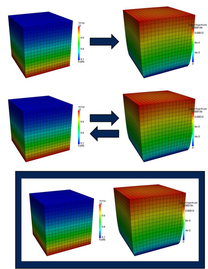
Figure 40: 耦合图
\[\begin{aligned} R_1(u_1, u_2) &= 0 \\ R_2(u_1, u_2) &= 0 \end{aligned}\]
\[\begin{pmatrix} \frac{\partial R_1}{\partial u_1} & \frac{\partial R_1}{\partial u_2} \\ \frac{\partial R_2}{\partial u_1} & \frac{\partial R_2}{\partial u_2} \end{pmatrix}\]
\[\begin{pmatrix} \frac{\partial R_1}{\partial u_1} & \mathbf{0} \\ \mathbf{0} & \frac{\partial R_2}{\partial u_2} \end{pmatrix}\]
55.2. MultiApp 层次结构
每个“app”被认为是一个独立的求解,并且总是有一个“主”app 驱动仿真。
- “主”(或“父”)app 可以有任意数量的 `MultiApp` 对象
- 每个 `MultiApp` 可以代表许多子应用程序(“子-apps”或“子”apps)
每个子-app 可以求解与主应用程序不同的物理。
- 子-app 可以是另一个 MOOSE 应用程序或外部应用程序
- 子-app 可以有 `MultiApps`,从而创建多级求解
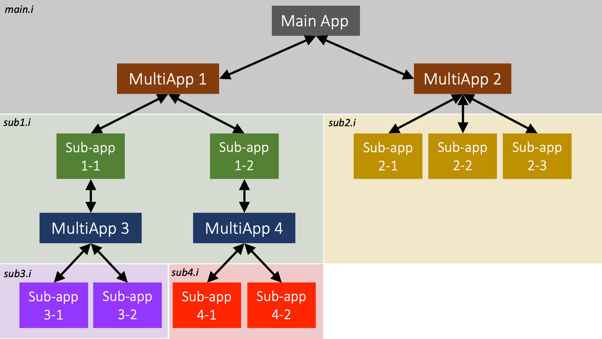
Figure 41: MultiApp 层次结构图
55.3. 输入文件语法
`MultiApp` 对象在 `[MultiApps]` 块中声明。
- `apptype`: 要运行的 `MooseApp` 派生应用程序的名称(例如,“AnimalApp”)
- `positions`: 描述子应用程序在主应用程序物理空间中偏移的 3D 坐标列表
- `executeon`: 允许控制子应用程序的执行时间:`INITIAL`, `LINEAR`, `NONLINEAR`, `TIMESTEPBEGIN`, `TIMESTEPEND`
- `inputfiles`: 可以为所有子应用程序提供一个输入文件,也可以为每个子应用程序提供一个文件
[MultiApps]
  [micro]
    type = TransientMultiApp
    app_type = DarcyThermoMechApp
    positions = '0.01285 0.0    0
                0.01285 0.0608 0
                0.01285 0.1216 0
                0.01285 0.1824 0
                0.01285 0.2432 0
                0.01285 0.304  0'
    input_files = step10_micro.i
    execute_on = 'timestep_end'
  []
[]
55.4. 并行
MultiApp 系统专为高效并行执行分层问题而设计。
- 主应用程序利用所有处理器
- 处理器在每个 MultiApp 中的每个子应用程序之间分配,并同时运行
- 多个 MultiApps 将
Generated org 一个接一个地执行
56. 传输系统
一个用于在 `MultiApp` 的“父应用程序”和“子应用程序”之间移动数据的系统。
新功能:传输现在可以在子应用程序之间发送数据。我们将此功能称为“兄弟”传输。
传输的数据通常由 `Auxiliary` 和 `Postprocessor` 系统接收。
接收应用程序上的数据应以正常方式耦合到这些值,并且每个子应用程序都应该能够独立求解。
56.1. 场传输
可以使用各种插值算法在应用程序之间传输场。
- 传输方向通过指定 `frommultiapp` 或 `tomultiapp` 参数来指定。
- 源场在目标点(通常是节点或单元质心,取决于接收变量类型)处进行评估。
- 然后将评估结果放入由 `variable` 参数指定的接收 `AuxVariable` 场中。
- `GeneralField` 版本的每种传输都是使用不同的算法实现的,并且可能更受欢迎,因为它们支持更多功能。
[Transfers]
  [from_sub]
    source_variable = sub_u
    variable = transferred_u
    type = MultiAppGeneralFieldShapeEvaluationTransfer
    from_multi_app = sub
    execute_on = 'initial timestep_end'
    # Test features non-overlapping meshes
    error_on_miss = false
  []
  [elemental_from_sub]
    source_variable = sub_u
    variable = elemental_transferred_u
    type = MultiAppGeneralFieldShapeEvaluationTransfer
    from_multi_app = sub
    # Test features non-overlapping meshes
    error_on_miss = false
  []
[]
56.2. UserObject 插值
- 许多 `UserObjects` 计算与网格不直接关联的空间变化数据。例如,功率变量的局部针状平均值。
- 任何 `UserObject` 都可以重写 `Real spatialValue(Point &)` 来提供给定空间点的值。
- `UserObjectTransfer` 可以从一个应用程序采样此空间变化的数据,并将值放入另一个应用程序的 `AuxVariable` 中。
- 此传输的 `GeneralField` 版本是使用不同的算法实现的,并且可能更受欢迎,因为它功能更全。
[Transfers]
  [layered_transfer_to_sub_app]
    type = MultiAppUserObjectTransfer
    user_object = main_uo
    variable = sub_app_var
    to_multi_app = sub_app
    displaced_target_mesh = true
  []
  [layered_transfer_from_sub_app]
    type = MultiAppUserObjectTransfer
    user_object = sub_app_uo
    variable = from_sub_app_var
    from_multi_app = sub_app
    displaced_source_mesh = true
  []
[]
56.3. 标量数传输
`Postprocessor` 或标量变量传输允许在应用程序之间传输标量值。
- 当传输到 `MultiApp` 时,该值可以放入 `Postprocessor` 值中,也可以放入 `constantAuxVariable` 场中——例如,子应用程序位置处的主应用程序变量值可以存储在后处理器中。
- 当从 `MultiApp` 传输到父应用程序时,可以将所有子应用程序的 `Postprocessor` 值插值以在父应用程序上形成辅助场。
[Transfers]
  [pp_transfer]
    type = MultiAppPostprocessorTransfer
    to_multi_app = pp_sub
    from_postprocessor = average
    to_postprocessor = from_parent
  []
[]
57. 第 10 步:多尺度仿真
57.1. (续)
57.2. RandomCorrosion.h
#pragma once

// MOOSE includes
#include "AuxKernel.h"
#include "libmesh/bounding_box.h"

/**
 * Creates artificial, temperature driven corrosion.
 *
 * Consider a multi-phase system represented by a field-variable varying
 * from 0 to 1. This class randomly sets points within the field to have
 * a value of 0. Additionally, there is a contrived relationship with the
 * number of points where "corrosion" occurs, the greater the difference
 * between the supplied postprocessor and the reference the more points
 * that are used.
 */
class RandomCorrosion : public AuxKernel
{
public:
  static InputParameters validParams();

  /**
   * Class constructor
   * @param parameters The input parameters for the RandomCorrosion object.
   */
  RandomCorrosion(const InputParameters & parameters);

  /**
   * At each timestep randomly create a vector of points to apply "corrosion".
   */
  void timestepSetup() override;

protected:
  /**
   * Computes the "corrosion" for the supplied phase variable.
   * @return The compute "phase" variable
   */
  virtual Real computeValue() override;

  /**
   * A helper method for getting random points in the domiain.
   * @return A random point within the bounding box of the domain
   */
  Point getRandomPoint();

private:
  /// The vector of random points to apply "corrosion"
  std::vector<Point> _points;

  /// The bounding box of the domain, used for generating "corrosion" points
  BoundingBox _box;

  /// Nodal tolerance for determining if "corrosion" should occur at the current node
  const Real & _nodal_tol;

  /// Minimum  number of "corrosion" points to apply
  const unsigned int & _num_points;

  /// Reference temperature, used for creating a temperature dependence and corrosion
  const Real & _ref_temperature;

  /// System temperature, used for creating a temperature dependence and corrosion
  const PostprocessorValue & _temperature;
};
57.3. RandomCorrosion.C
// MOOSE includes
#include "RandomCorrosion.h"
#include "MooseMesh.h"

#include "libmesh/mesh_tools.h"

registerMooseObject("DarcyThermoMechApp", RandomCorrosion);

InputParameters
RandomCorrosion::validParams()
{
  InputParameters params = AuxKernel::validParams();
  params.addParam<Real>("tolerance",
                        1e-3,
                        "When acting as a nodal AuxKernel determine if the "
                        "random point to apply corrosion is located at the "
                        "current node.");
  params.addParam<unsigned int>("num_points",
                                10,
                                "The number of random points to apply artificial "
                                "corrosion. The number of points is increased by "
                                "a factor as the supplied temperatures diverge.");
  params.addParam<Real>("reference_temperature",
                        273.15,
                        "Temperature at which corrosion begins, "
                        "the greater the 'temperature' drifts "
                        "from this the greater the amount of "
                        "corrosion locations that occurs.");
  params.addParam<PostprocessorName>(
      "temperature",
      274.15,
      "The temperature value to used for computing the temperature "
      "multiplication factor for the number of corrosion locations.");
  return params;
}

RandomCorrosion::RandomCorrosion(const InputParameters & parameters)
  : AuxKernel(parameters),
    _box(MeshTools::create_bounding_box(_mesh)),
    _nodal_tol(getParam<Real>("tolerance")),
    _num_points(getParam<unsigned int>("num_points")),
    _ref_temperature(getParam<Real>("reference_temperature")),
    _temperature(getPostprocessorValue("temperature"))
{
  // This class only works with Nodal aux variables
  if (!isNodal())
    mooseError("RandomCorrosion only operates using nodal aux variables.");

  // Setup the random number generation
  setRandomResetFrequency(EXEC_TIMESTEP_BEGIN);
}

void
RandomCorrosion::timestepSetup()
{
  // Increase the number of points as the temperature differs from the reference
  Real factor = 1;
  if (_temperature > _ref_temperature)
    factor = 1 + (_temperature - _ref_temperature) * 0.1;

  // Generater the random points to apply "corrosion"
  _points.clear();
  for (unsigned int i = 0; i < _num_points * factor; ++i)
    _points.push_back(getRandomPoint());
}

Real
RandomCorrosion::computeValue()
{

  // If the current node is at a "corrosion" point, set the phase variable to zero
  for (const Point & pt : _points)
    if (_current_node->absolute_fuzzy_equals(pt, _nodal_tol))
      return 0.0;

  // Do nothing to the phase variable if not at a "corrosion" point
  return _u[_qp];
}

Point
RandomCorrosion::getRandomPoint()
{
  // Generates a random point within the domain
  const Point & min = _box.min();
  const Point & max = _box.max();

  Real x = getRandomReal() * (max(0) - min(0)) + min(0);
  Real y = getRandomReal() * (max(1) - min(1)) + min(1);
  Real z = getRandomReal() * (max(2) - min(2)) + min(2);

  return Point(x, y, z);
}
57.4. 第 10 步:微观尺度输入文件
[Mesh]
  [gmg]
    type = GeneratedMeshGenerator
    dim = 2
    nx = 10
    ny = 10
    ymax = 0.1
    xmax = 0.1
  []

  uniform_refine = 0
[]

[Adaptivity]
  max_h_level = 4
  initial_steps = 6
  initial_marker = error_marker
  cycles_per_step = 2
  marker = error_marker
  [Indicators/phi_jump]
    type = GradientJumpIndicator
    variable = phi
  []
  [Markers/error_marker]
    type = ErrorFractionMarker
    indicator = phi_jump
    refine = 0.8
    coarsen = 0.1
  []
[]

[Variables/temperature]
  initial_condition = 300
[]

[AuxVariables/phi]
[]

[AuxKernels/corrosion]
  type = RandomCorrosion
  variable = phi
  reference_temperature = 300
  temperature = temperature_in
  execute_on = 'INITIAL TIMESTEP_END'
[]

[Kernels/heat_conduction]
  type = ADHeatConduction
  variable = temperature
[]

[BCs]
  [left]
    type = PostprocessorDirichletBC
    variable = temperature
    boundary = left
    postprocessor = temperature_in
  []
  [right]
    type = NeumannBC
    variable = temperature
    boundary = right
    value = 100 # prescribed flux
  []
[]

[Materials/column]
  type = PackedColumn
  temperature = temperature
  radius = 1 # mm
  phase = phi
[]

[Postprocessors]
  [temperature_in]
    type = Receiver
    default = 301
  []
  [k_eff]
    type = ThermalConductivity
    variable = temperature
    T_hot = temperature_in
    flux = 100
    dx = 0.1
    boundary = right
    length_scale = 1
    k0 = 12.05
    execute_on = 'INITIAL TIMESTEP_END'
  []
  [average_porosity]
    type = ADElementAverageMaterialProperty
    mat_prop = porosity
    execute_on = 'INITIAL TIMESTEP_END'
  []
  [t_right]
    type = SideAverageValue
    boundary = right
    variable = temperature
    execute_on = 'INITIAL TIMESTEP_END'
  []
[]

[Executioner]
  type = Transient
  end_time = 1000
  dt = 1
  steady_state_tolerance = 1e-9
  steady_state_detection = true
  solve_type = NEWTON
  petsc_options_iname = '-pc_type -pc_hypre_type'
  petsc_options_value = 'hypre boomeramg'
  automatic_scaling = true
[]

[Outputs]
  execute_on = 'initial timestep_end'
  exodus = true
[]

[ICs/close_pack]
  radius = 0.01 # meter
  outvalue = 0 # water
  variable = phi
  invalue = 1 # steel
  type = ClosePackIC
[]
57.5. 第 10 步:运行微观尺度
cd ~/projects/moose/tutorials/darcy_thermo_mech/step10_multiapps
make -j 12 # 使用您系统的处理器数量
cd problems
../darcy_thermo_mech-opt  -i step10_micro.i
57.6. 第 10 步:微观尺度结果
57.7. PackedColumn.h
 @@ -1,108 +1,120 @@

 #pragma once

 #include "Material.h"

 // A helper class from MOOSE that linear interpolates x,y data
 #include "LinearInterpolation.h"

 /**
  * Material objects inherit from Material and override computeQpProperties.
  *
  * Their job is to declare properties for use by other objects in the
  * calculation such as Kernels and BoundaryConditions.
  */
 class PackedColumn : public Material
 {
 public:
   static InputParameters validParams();

   PackedColumn(const InputParameters & parameters);

 protected:
   /// Necessary override. This is where the values of the properties are computed.
   virtual void computeQpProperties() override;

   /**
    * Helper function for reading CSV data for use in an interpolator object.
    */
   bool initInputData(const std::string & param_name, ADLinearInterpolation & interp);

   /// The radius of the spheres in the column
   const Function & _input_radius;

   /// The input porosity
   const Function & _input_porosity;

   /// Temperature
   const ADVariableValue & _temperature;

   /// Compute permeability based on the radius (mm)
   LinearInterpolation _permeability_interpolation;

   /// Fluid viscosity
   bool _use_fluid_mu_interp;
   const Real & _fluid_mu;
   ADLinearInterpolation _fluid_mu_interpolation;

   /// Fluid thermal conductivity
   bool _use_fluid_k_interp = false;
   const Real & _fluid_k;
   ADLinearInterpolation _fluid_k_interpolation;

   /// Fluid density
   bool _use_fluid_rho_interp = false;
   const Real & _fluid_rho;
   ADLinearInterpolation _fluid_rho_interpolation;

   /// Fluid specific heat
   bool _use_fluid_cp_interp;
   const Real & _fluid_cp;
   ADLinearInterpolation _fluid_cp_interpolation;

   /// Fluid thermal expansion coefficient
   bool _use_fluid_cte_interp;
   const Real & _fluid_cte;
   ADLinearInterpolation _fluid_cte_interpolation;

   /// Solid thermal conductivity
   bool _use_solid_k_interp = false;
   const Real & _solid_k;
   ADLinearInterpolation _solid_k_interpolation;

   /// Solid density
   bool _use_solid_rho_interp = false;
   const Real & _solid_rho;
   ADLinearInterpolation _solid_rho_interpolation;

   /// Solid specific heat
   bool _use_solid_cp_interp;
   const Real & _solid_cp;
   ADLinearInterpolation _solid_cp_interpolation;

   /// Solid thermal expansion coefficient
   bool _use_solid_cte_interp;
   const Real & _solid_cte;
   ADLinearInterpolation _solid_cte_interpolation;

   /// The permeability (K)
   ADMaterialProperty<Real> & _permeability;

   /// The viscosity of the fluid (mu)
   ADMaterialProperty<Real> & _viscosity;

   /// The porosity (eps)
   ADMaterialProperty<Real> & _porosity;

   /// The bulk thermal conductivity
   ADMaterialProperty<Real> & _thermal_conductivity;

   /// The bulk heat capacity
   ADMaterialProperty<Real> & _specific_heat;

   /// The bulk density
   ADMaterialProperty<Real> & _density;

   /// The bulk thermal expansion coefficient
   ADMaterialProperty<Real> & _thermal_expansion;
+
+  /// Flag for using the phase for porosity
+  bool _use_phase_variable;
+
+  /// The coupled phase variable
+  const VariableValue & _phase;
+
+  /// Flag for using a variable for thermal conductivity
+  bool _use_variable_conductivity;
+
+  /// The coupled thermal conductivity
+  const VariableValue & _conductivity_variable;
 };
57.8. PackedColumn.C
 @@ -1,201 +1,232 @@

 #include "PackedColumn.h"
 #include "Function.h"
 #include "DelimitedFileReader.h"

 registerMooseObject("DarcyThermoMechApp", PackedColumn);

 InputParameters
 PackedColumn::validParams()
 {
   InputParameters params = Material::validParams();
   params.addRequiredCoupledVar("temperature", "The temperature (C) of the fluid.");

   // Parameter for radius of the spheres used to interpolate permeability.
   params.addParam<FunctionName>("radius",
                                 "1.0",
                                 "The radius of the steel spheres (mm) that are packed in the "
                                 "column for computing permeability.");

   // http://en.wikipedia.org/wiki/Close-packing_of_equal_spheres
   params.addParam<FunctionName>(
       "porosity", 0.25952, "Porosity of porous media, default is for closed packed spheres.");

   // Fluid properties
   params.addParam<Real>(
       "fluid_viscosity", 1.002e-3, "Fluid viscosity (Pa s); default is for water at 20C).");
   params.addParam<FileName>(
       "fluid_viscosity_file",
       "The name of a file containing the fluid viscosity (Pa-s) as a function of temperature "
       "(C); if provided the constant value is ignored.");

   params.addParam<Real>("fluid_thermal_conductivity",
                         0.59803,
                         "Fluid thermal conductivity (W/(mK); default is for water at 20C).");
   params.addParam<FileName>(
       "fluid_thermal_conductivity_file",
       "The name of a file containing fluid thermal conductivity (W/(mK)) as a function of "
       "temperature (C); if provided the constant value is ignored.");

   params.addParam<Real>(
       "fluid_density", 998.21, "Fluid density (kg/m^3); default is for water at 20C).");
   params.addParam<FileName>("fluid_density_file",
                             "The name of a file containing fluid density (kg/m^3) as a function "
                             "of temperature (C); if provided the constant value is ignored.");

   params.addParam<Real>(
       "fluid_specific_heat", 4157.0, "Fluid specific heat (J/(kgK); default is for water at 20C).");
   params.addParam<FileName>(
       "fluid_specific_heat_file",
       "The name of a file containing fluid specific heat (J/(kgK) as a function of temperature "
       "(C); if provided the constant value is ignored.");

   params.addParam<Real>("fluid_thermal_expansion",
                         2.07e-4,
                         "Fluid thermal expansion coefficient (1/K); default is for water at 20C).");
   params.addParam<FileName>("fluid_thermal_expansion_file",
                             "The name of a file containing fluid thermal expansion coefficient "
                             "(1/K) as a function of temperature "
                             "(C); if provided the constant value is ignored.");

   // Solid properties
   // https://en.wikipedia.org/wiki/Stainless_steel#Properties
   params.addParam<Real>("solid_thermal_conductivity",
                         15.0,
                         "Solid thermal conductivity (W/(mK); default is for AISI/ASTIM 304 "
                         "stainless steel at 20C).");
   params.addParam<FileName>(
       "solid_thermal_conductivity_file",
       "The name of a file containing solid thermal conductivity (W/(mK)) as a function of "
       "temperature (C); if provided the constant value is ignored.");

   params.addParam<Real>(
       "solid_density",
       7900,
       "Solid density (kg/m^3); default is for AISI/ASTIM 304 stainless steel at 20C).");
   params.addParam<FileName>("solid_density_file",
                             "The name of a file containing solid density (kg/m^3) as a function "
                             "of temperature (C); if provided the constant value is ignored.");

   params.addParam<Real>(
       "solid_specific_heat",
       500,
       "Solid specific heat (J/(kgK); default is for AISI/ASTIM 304 stainless steel at 20C).");
   params.addParam<FileName>(
       "solid_specific_heat_file",
       "The name of a file containing solid specific heat (J/(kgK) as a function of temperature "
       "(C); if provided the constant value is ignored.");

   params.addParam<Real>("solid_thermal_expansion",
                         17.3e-6,
                         "Solid thermal expansion coefficient (1/K); default is for water at 20C).");
   params.addParam<FileName>("solid_thermal_expansion_file",
                             "The name of a file containing solid thermal expansion coefficient "
                             "(1/K) as a function of temperature "
                             "(C); if provided the constant value is ignored.");
+
+  // Optional phase variable
+  params.addCoupledVar("phase",
+                       "The variable indicating the phase (steel=1 or water=0). If "
+                       "supplied this is used to compute the porosity instead of the "
+                       "supplied value.");
+
+  // Optional thermal conductivity variable
+  params.addCoupledVar("thermal_conductivity",
+                       "When supplied the variable be will be used for "
+                       "thermal conductivity rather than being computed.");
   return params;
 }

 PackedColumn::PackedColumn(const InputParameters & parameters)
   : Material(parameters),

     // Get the parameters from the input file
     _input_radius(getFunction("radius")),
     _input_porosity(getFunction("porosity")),
     _temperature(adCoupledValue("temperature")),

     // Fluid
     _fluid_mu(getParam<Real>("fluid_viscosity")),
     _fluid_k(getParam<Real>("fluid_thermal_conductivity")),
     _fluid_rho(getParam<Real>("fluid_density")),
     _fluid_cp(getParam<Real>("fluid_specific_heat")),
     _fluid_cte(getParam<Real>("fluid_thermal_expansion")),

     // Solid
     _solid_k(getParam<Real>("solid_thermal_conductivity")),
     _solid_rho(getParam<Real>("solid_density")),
     _solid_cp(getParam<Real>("solid_specific_heat")),
     _solid_cte(getParam<Real>("solid_thermal_expansion")),

     // Material Properties being produced by this object
     _permeability(declareADProperty<Real>("permeability")),
     _viscosity(declareADProperty<Real>("viscosity")),
     _porosity(declareADProperty<Real>("porosity")),
     _thermal_conductivity(declareADProperty<Real>("thermal_conductivity")),
     _specific_heat(declareADProperty<Real>("specific_heat")),
     _density(declareADProperty<Real>("density")),
-    _thermal_expansion(declareADProperty<Real>("thermal_expansion"))
+    _thermal_expansion(declareADProperty<Real>("thermal_expansion")),
+
+    // Optional phase variable
+    _use_phase_variable(isParamValid("phase")),
+    _phase(_use_phase_variable ? coupledValue("phase") : _zero),
+
+    // Optional thermal conductivity variable
+    _use_variable_conductivity(isParamValid("thermal_conductivity")),
+    _conductivity_variable(_use_variable_conductivity ? coupledValue("thermal_conductivity")
+                                                      : _zero)
 {
   // Set data for permeability interpolation
   std::vector<Real> sphere_sizes = {1, 3};
   std::vector<Real> permeability = {0.8451e-9, 8.968e-9};
   _permeability_interpolation.setData(sphere_sizes, permeability);

   // Fluid viscosity, thermal conductivity, density, and specific heat
   _use_fluid_mu_interp = initInputData("fluid_viscosity_file", _fluid_mu_interpolation);
   _use_fluid_k_interp = initInputData("fluid_thermal_conductivity_file", _fluid_k_interpolation);
   _use_fluid_rho_interp = initInputData("fluid_density_file", _fluid_rho_interpolation);
   _use_fluid_cp_interp = initInputData("fluid_specific_heat_file", _fluid_cp_interpolation);
   _use_fluid_cte_interp = initInputData("fluid_thermal_expansion_file", _fluid_cte_interpolation);

   // Solid thermal conductivity, density, and specific heat
   _use_solid_k_interp = initInputData("solid_thermal_conductivity_file", _solid_k_interpolation);
   _use_solid_rho_interp = initInputData("solid_density_file", _solid_rho_interpolation);
   _use_solid_cp_interp = initInputData("solid_specific_heat_file", _solid_cp_interpolation);
   _use_solid_cte_interp = initInputData("solid_thermal_expansion_file", _solid_cte_interpolation);
 }

 void
 PackedColumn::computeQpProperties()
 {
   // Current temperature
   ADReal temp = _temperature[_qp] - 273.15;

   // Permeability
   Real radius_value = _input_radius.value(_t, _q_point[_qp]);
   mooseAssert(radius_value >= 1 && radius_value <= 3,
               "The radius range must be in the range [1, 3], but " << radius_value << " provided.");
   _permeability[_qp] = _permeability_interpolation.sample(radius_value);

   // Porosity
-  Real porosity_value = _input_porosity.value(_t, _q_point[_qp]);
-  mooseAssert(porosity_value > 0 && porosity_value <= 1,
-              "The porosity range must be in the range (0, 1], but " << porosity_value
-                                                                     << " provided.");
-  _porosity[_qp] = porosity_value;
+  if (_use_phase_variable)
+    _porosity[_qp] = 1 - _phase[_qp];
+  else
+  {
+    Real porosity_value = _input_porosity.value(_t, _q_point[_qp]);
+    mooseAssert(porosity_value > 0 && porosity_value <= 1,
+                "The porosity range must be in the range (0, 1], but " << porosity_value
+                                                                       << " provided.");
+    _porosity[_qp] = porosity_value;
+  }

   // Fluid properties
   _viscosity[_qp] = _use_fluid_mu_interp ? _fluid_mu_interpolation.sample(temp) : _fluid_mu;
-  ADReal fluid_k = _use_fluid_k_interp ? _fluid_k_interpolation.sample(temp) : _fluid_k;
   ADReal fluid_rho = _use_fluid_rho_interp ? _fluid_rho_interpolation.sample(temp) : _fluid_rho;
   ADReal fluid_cp = _use_fluid_cp_interp ? _fluid_cp_interpolation.sample(temp) : _fluid_cp;
   ADReal fluid_cte = _use_fluid_cte_interp ? _fluid_cte_interpolation.sample(temp) : _fluid_cte;

   // Solid properties
-  ADReal solid_k = _use_solid_k_interp ? _solid_k_interpolation.sample(temp) : _solid_k;
   ADReal solid_rho = _use_solid_rho_interp ? _solid_rho_interpolation.sample(temp) : _solid_rho;
   ADReal solid_cp = _use_solid_cp_interp ? _solid_cp_interpolation.sample(temp) : _solid_cp;
   ADReal solid_cte = _use_solid_cte_interp ? _solid_cte_interpolation.sample(temp) : _solid_cte;

   // Compute the heat conduction material properties as a linear combination of
   // the material properties for fluid and steel.
-  _thermal_conductivity[_qp] = _porosity[_qp] * fluid_k + (1.0 - _porosity[_qp]) * solid_k;
+  if (_use_variable_conductivity)
+    _thermal_conductivity[_qp] = _conductivity_variable[_qp];
+  else
+  {
+    ADReal fluid_k = _use_fluid_k_interp ? _fluid_k_interpolation.sample(temp) : _fluid_k;
+    ADReal solid_k = _use_solid_k_interp ? _solid_k_interpolation.sample(temp) : _solid_k;
+    _thermal_conductivity[_qp] = _porosity[_qp] * fluid_k + (1.0 - _porosity[_qp]) * solid_k;
+  }
+
   _density[_qp] = _porosity[_qp] * fluid_rho + (1.0 - _porosity[_qp]) * solid_rho;
   _specific_heat[_qp] = _porosity[_qp] * fluid_cp + (1.0 - _porosity[_qp]) * solid_cp;
   _thermal_expansion[_qp] = _porosity[_qp] * fluid_cte + (1.0 - _porosity[_qp]) * solid_cte;
 }

 bool
 PackedColumn::initInputData(const std::string & param_name, ADLinearInterpolation & interp)
 {
   if (isParamValid(param_name))
   {
     const std::string & filename = getParam<FileName>(param_name);
     MooseUtils::DelimitedFileReader reader(filename, &_communicator);
     reader.setComment("#");
     reader.read();
     interp.setData(reader.getData(0), reader.getData(1));
     return true;
   }
   return false;
 }
57.9. 第 10 步:多尺度输入文件
 @@ -1,202 +1,220 @@
-[GlobalParams]
+[GlobalParams]
   displacements = 'disp_r disp_z'
 []

 [Mesh]
   [gmg]
     type = GeneratedMeshGenerator
     dim = 2
     nx = 10
-    ny = 200
+    ny = 100
     ymax = 0.304 # Length of test chamber
     xmax = 0.0257 # Test chamber radius
   []
--  [bottom]
--    type = SubdomainBoundingBoxGenerator
--    input = gmg
--    location = inside
--    bottom_left = '0 0 0'
--    top_right = '0.01285 0.304 0'
--    block_id = 1
--  []
-  coord_type = RZ
 []

 [Variables]
   [pressure]
   []
   [temperature]
-    initial_condition = 300 # Start at room temperature
-  []
-[]
-
-[Physics/SolidMechanics/QuasiStatic]
+    initial_condition = 300
+  []
+[]
+
+[Physics/SolidMechanics/QuasiStatic]
   [all]
     # This block adds all of the proper Kernels, strain calculators, and Variables
     # for SolidMechanics in the correct coordinate system (autodetected)
-    add_variables = true
-    strain = FINITE
-    eigenstrain_names = eigenstrain
-    use_automatic_differentiation = true
-    generate_output = 'vonmises_stress elastic_strain_xx elastic_strain_yy strain_xx strain_yy'
-  []
-[]
-
-[Kernels]
-  [darcy_pressure]
-    type = DarcyPressure
-    variable = pressure
-  []
-  [heat_conduction]
-    type = ADHeatConduction
-    variable = temperature
-  []
-  [heat_conduction_time_derivative]
-    type = ADHeatConductionTimeDerivative
-    variable = temperature
-  []
-  [heat_convection]
-    type = DarcyAdvection
-    variable = temperature
-    pressure = pressure
-  []
-[]
-
+    add_variables = true
+    strain = FINITE
+    eigenstrain_names = eigenstrain
+    use_automatic_differentiation = true
+    generate_output = 'vonmises_stress elastic_strain_xx elastic_strain_yy strain_xx strain_yy'
+  []
+[]
+
+[Kernels]
+  [darcy_pressure]
+    type = DarcyPressure
+    variable = pressure
+  []
+  [heat_conduction]
+    type = ADHeatConduction
+    variable = temperature
+  []
+  [heat_conduction_time_derivative]
+    type = ADHeatConductionTimeDerivative
+    variable = temperature
+  []
+  [heat_convection]
+    type = DarcyAdvection
+    variable = temperature
+    pressure = pressure
+  []
+[]
+
 [BCs]
   [inlet_temperature]
-    type = FunctionDirichletBC
-    variable = temperature
-    boundary = bottom
-    function = 'if(t<0,350+50*t,350)'
+    type = FunctionDirichletBC
+    variable = temperature
+    boundary = bottom
+    function = 'if(t<0,350+50*t,350)'
   []
   [outlet_temperature]
     type = HeatConductionOutflow
     variable = temperature
     boundary = top
   []
   [inlet]
-    type = DirichletBC
-    variable = pressure
-    boundary = bottom
-    value = 4000 # (Pa) From Figure 2 from paper.  First data point for 1mm spheres.
+    type = DirichletBC
+    variable = pressure
+    boundary = bottom
+    value = 4000
   []
   [outlet]
-    type = DirichletBC
-    variable = pressure
-    boundary = top
-    value = 0 # (Pa) Gives the correct pressure drop from Figure 2 for 1mm spheres.
+    type = DirichletBC
+    variable = pressure
+    boundary = top
+    value = 0
   []
   [hold_inlet]
-    type = DirichletBC
-    variable = disp_z
-    boundary = bottom
-    value = 0
+    type = DirichletBC
+    variable = disp_z
+    boundary = bottom
+    value = 0
   []
   [hold_center]
-    type = DirichletBC
-    variable = disp_r
-    boundary = left
-    value = 0
+    type = DirichletBC
+    variable = disp_r
+    boundary = left
+    value = 0
   []
   [hold_outside]
-    type = DirichletBC
-    variable = disp_r
-    boundary = right
-    value = 0
-  []
-[]
-
-[Materials]
+    type = DirichletBC
+    variable = disp_r
+    boundary = right
+    value = 0
+  []
+[]
+
+[Materials]
   viscosity_file = data/water_viscosity.csv
   density_file = data/water_density.csv
--  thermal_conductivity_file = data/water_thermal_conductivity.csv
   specific_heat_file = data/water_specific_heat.csv
   thermal_expansion_file = data/water_thermal_expansion.csv
 -
-  [column_top]
+  [column]
     type = PackedColumn
--    block = 0
     temperature = temperature
-    radius = 1.15
+    radius = 1
+    thermal_conductivity = k_eff # Use the AuxVariable instead of calculating
     fluid_viscosity_file = ${viscosity_file}
     fluid_density_file = ${density_file}
--    fluid_thermal_conductivity_file = ${thermal_conductivity_file}
--    fluid_specific_heat_file = ${specific_heat_file}
--    fluid_thermal_expansion_file = ${thermal_expansion_file}
--  []
--  [column_bottom]
--    type = PackedColumn
--    block = 1
--    temperature = temperature
--    radius = 1
--    fluid_viscosity_file = ${viscosity_file}
--    fluid_density_file = ${density_file}
--    fluid_thermal_conductivity_file = ${thermal_conductivity_file}
     fluid_specific_heat_file = ${specific_heat_file}
     fluid_thermal_expansion_file = ${thermal_expansion_file}
   []

   [elasticity_tensor]
-    type = ADComputeIsotropicElasticityTensor
-    youngs_modulus = 200e9 # (Pa) from wikipedia
-    poissons_ratio = .3 # from wikipedia
+    type = ADComputeIsotropicElasticityTensor
+    youngs_modulus = 200e9
+    poissons_ratio = .3
   []
   [elastic_stress]
-    type = ADComputeFiniteStrainElasticStress
+    type = ADComputeFiniteStrainElasticStress
   []
   [thermal_strain]
-    type = ADComputeThermalExpansionEigenstrain
-    stress_free_temperature = 300
-    eigenstrain_name = eigenstrain
-    temperature = temperature
-    thermal_expansion_coeff = 1e-5
-  []
-[]
-
-[Postprocessors/average_temperature]
-  type = ElementAverageValue
-  variable = temperature
+    type = ADComputeThermalExpansionEigenstrain
+    stress_free_temperature = 300
+    eigenstrain_name = eigenstrain
+    temperature = temperature
+    thermal_expansion_coeff = 1e-6
+  []
+[]
+
+[Postprocessors/average_temperature]
+  type = ElementAverageValue
+  variable = temperature
 []

 [AuxVariables/velocity]
   order = CONSTANT
   family = MONOMIAL_VEC
+[]
+[AuxVariables/k_eff] # filled from the multiapp
+  initial_condition = 15.0 # water at 20C
 []

 [AuxKernels/velocity]
   type = DarcyVelocity
   variable = velocity
   execute_on = timestep_end
   pressure = pressure
 []

 [Problem]
   type = FEProblem
 []

 [Executioner]
   type = Transient
   end_time = 200
   dt = 0.25
   start_time = -1

   solve_type = PJFNK
--  petsc_options_iname = '-pc_type'
--  petsc_options_value = 'lu'
+  petsc_options_iname = '-pc_type -pc_hypre_type -ksp_gmres_restart'
+  petsc_options_value = 'hypre boomeramg 500'
   line_search = none

   automatic_scaling = true
   compute_scaling_once = false
   steady_state_tolerance = 1e-7
   steady_state_detection = true

   [TimeStepper]
     type = FunctionDT
     function = 'if(t<0,0.1,0.25)'
   []
 []

+[MultiApps/micro]
+  type = TransientMultiApp
+  app_type = DarcyThermoMechApp
+  positions = '0.01285 0.0    0
+                0.01285 0.0608 0
+                0.01285 0.1216 0
+                0.01285 0.1824 0
+                0.01285 0.2432 0
+                0.01285 0.304  0'
+  input_files = step10_micro.i
+  execute_on = 'timestep_end'
+[]
+
+[Transfers]
+  [keff_from_sub]
+    type = MultiAppPostprocessorInterpolationTransfer
+    from_multi_app = micro
+    variable = k_eff
+    power = 1
+    postprocessor = k_eff
+    execute_on = 'timestep_end'
+  []
+  [temperature_to_sub]
+    type = MultiAppVariableValueSamplePostprocessorTransfer
+    to_multi_app = micro
+    source_variable = temperature
+    postprocessor = temperature_in
+    execute_on = 'timestep_end'
+  []
+[]
+
+[Controls/multiapp]
+  type = TimePeriod
+  disable_objects = 'MultiApps::micro Transfers::keff_from_sub Transfers::temperature_to_sub'
+  start_time = '0'
+  execute_on = 'initial'
+[]
+
 [Outputs/out]
-  type = Exodus
-  elemental_as_nodal = true
+  type = Exodus
+  elemental_as_nodal = true
 []
57.10. 第 10 步:运行多尺度
cd ~/projects/moose/tutorials/darcy_thermo_mech/step10_multiapps
make -j 12 # 使用您系统的处理器数量
cd problems
../darcy_thermo_mech-opt -i step10.i
58. 第 11 步:自定义语法
为所有达西热力学问题中常见的对象添加自定义语法:
- 速度辅助变量和内核
- 压力内核
- 温度内核
59. Action 系统
一个用于以编程方式创建仿真对象和输入文件语法的系统。
59.1. 创建 Action
继承自 `Action` 或 `MooseObjectAction` 并重写 `act()` 方法。
注意,构造函数使用 `InputParameters` 对象的副本。这是设计使然,以便在对象创建期间可以操作和重用参数。
59.2. Action 对象
一个旨在构建特定对象的 action,如第 9 步:力学中固体力学的情况。
[Physics]
  [SolidMechanics]
    [QuasiStatic]
      [all]
        # This block adds all of the proper Kernels, strain calculators, and Variables
        # for SolidMechanics in the correct coordinate system (autodetected)
        add_variables = true
        strain = FINITE
        eigenstrain_names = eigenstrain
        use_automatic_differentiation = true
        generate_output = 'vonmises_stress elastic_strain_xx elastic_strain_yy strain_xx strain_yy'
      []
    []
  []
[]
59.3. 语法和任务
MOOSE action 系统对任务进行操作,每个任务都与一个或多个 action 相关联。
对于每个任务,都会调用 `act()` 方法。因此,`act` 方法可用于创建任意数量的对象。
通常,在应用程序的 `registerAll` 方法中调用以下宏来创建构建所需对象的必要语法和任务。
- `registerSyntax(action, actionsyntax)`: 创建在 "actionsyntax" 中提供的输入文件语法,并与提供的 "action" 关联
- `registerSyntaxTask(action, actionsyntax, task)`: 与上面相同,但还创建一个将要执行的命名任务。
- `registerTask(name, isrequired)`: 创建一个可以与 action 关联的命名任务。
- `addTaskDependency(action, dependson)`: 在两个任务之间创建依赖关系,以帮助控制任务执行的顺序。
59.4. MooseObjectAction 对象
一个旨在构建一个或多个其他 `MooseObjects` 的 action,例如 `[Dampers]` 块的情况。
59.5. AddDamperAction.h
#pragma once

#include "MooseObjectAction.h"

class AddDamperAction : public MooseObjectAction
{
public:
  static InputParameters validParams();

  AddDamperAction(const InputParameters & params);

  virtual void act() override;
};
59.6. AddDamperAction.C
#include "AddDamperAction.h"
#include "FEProblem.h"

registerMooseAction("MooseApp", AddDamperAction, "add_damper");

InputParameters
AddDamperAction::validParams()
{
  InputParameters params = MooseObjectAction::validParams();
  params.addClassDescription("Add a Damper object to the simulation.");
  return params;
}

AddDamperAction::AddDamperAction(const InputParameters & params) : MooseObjectAction(params) {}

void
AddDamperAction::act()
{
  _problem->addDamper(_type, _name, _moose_object_pars);
}
59.7. Moose.C
registerSyntax("AddDamperAction", "Dampers/*");
60. 第 11 步:自定义语法
60.1. (续)
60.2. SetupDarcySimulation.h
#pragma once

// MOOSE includes
#include "Action.h"

/**
 * An action for creating the necessary objects to perform a thermal mechanics problem using
 * Darcy's equation.
 * */
class SetupDarcySimulation : public Action
{
public:
  static InputParameters validParams();

  SetupDarcySimulation(const InputParameters & params);
  virtual void act() override;

protected:
  const bool _compute_velocity;
  const bool _compute_pressure;
  const bool _compute_temperature;
};
60.3. SetupDarcySimulation.C
#include "SetupDarcySimulation.h"

// MOOSE includes
#include "FEProblem.h"
#include "AuxiliarySystem.h"

// libMesh includes
#include "libmesh/fe.h"

registerMooseAction("DarcyThermoMechApp", SetupDarcySimulation, "add_aux_variable");
registerMooseAction("DarcyThermoMechApp", SetupDarcySimulation, "add_aux_kernel");
registerMooseAction("DarcyThermoMechApp", SetupDarcySimulation, "add_kernel");

InputParameters
SetupDarcySimulation::validParams()
{
  InputParameters params = Action::validParams();
  params.addParam<VariableName>("pressure", "pressure", "The pressure variable.");
  params.addParam<VariableName>("temperature", "temperature", "The temperature variable.");
  params.addParam<bool>(
      "compute_velocity", true, "Enable the auxiliary calculation of velocity from pressure.");
  params.addParam<bool>("compute_pressure", true, "Enable the computation of pressure.");
  params.addParam<bool>("compute_temperature", true, "Enable the computation of temperature.");
  return params;
}

SetupDarcySimulation::SetupDarcySimulation(const InputParameters & parameters)
  : Action(parameters),
    _compute_velocity(getParam<bool>("compute_velocity")),
    _compute_pressure(getParam<bool>("compute_pressure")),
    _compute_temperature(getParam<bool>("compute_temperature"))
{
}

void
SetupDarcySimulation::act()
{
  // Actual names of input variables
  const std::string pressure = getParam<VariableName>("pressure");
  const std::string temperature = getParam<VariableName>("temperature");

  // Velocity AuxVariables
  if (_compute_velocity && _current_task == "add_aux_variable")
  {
    InputParameters var_params = _factory.getValidParams("VectorMooseVariable");
    var_params.set<MooseEnum>("family") = "MONOMIAL_VEC";
    var_params.set<MooseEnum>("order") = "CONSTANT";

    _problem->addAuxVariable("VectorMooseVariable", "velocity", var_params);
  }

  // Velocity AuxKernels
  else if (_compute_velocity && _current_task == "add_aux_kernel")
  {
    InputParameters params = _factory.getValidParams("DarcyVelocity");
    params.set<ExecFlagEnum>("execute_on") = EXEC_TIMESTEP_END;
    params.set<std::vector<VariableName>>("pressure") = {pressure};

    params.set<AuxVariableName>("variable") = "velocity";
    _problem->addAuxKernel("DarcyVelocity", "velocity", params);
  }

  // Kernels
  else if (_current_task == "add_kernel")
  {
    // Flags for aux variables
    const bool is_pressure_aux = _problem->getAuxiliarySystem().hasVariable(pressure);
    const bool is_temperature_aux = _problem->getAuxiliarySystem().hasVariable(temperature);

    // Pressure
    if (_compute_pressure && !is_pressure_aux)
    {
      InputParameters params = _factory.getValidParams("DarcyPressure");
      params.set<NonlinearVariableName>("variable") = pressure;
      _problem->addKernel("DarcyPressure", "darcy_pressure", params);
    }

    // Temperature
    if (_compute_temperature && !is_temperature_aux)
    {
      {
        InputParameters params = _factory.getValidParams("ADHeatConduction");
        params.set<NonlinearVariableName>("variable") = temperature;
        _problem->addKernel("ADHeatConduction", "heat_conduction", params);
      }

      {
        InputParameters params = _factory.getValidParams("ADHeatConductionTimeDerivative");
        params.set<NonlinearVariableName>("variable") = temperature;
        _problem->addKernel("ADHeatConductionTimeDerivative", "heat_conduction_time", params);
      }

      {
        InputParameters params = _factory.getValidParams("DarcyAdvection");
        params.set<NonlinearVariableName>("variable") = temperature;
        params.set<std::vector<VariableName>>("pressure") = {pressure};
        _problem->addKernel("DarcyAdvection", "heat_advection", params);
      }
    }
  }
}
60.4. DarcyThermoMechApp.h
#pragma once

#include "MooseApp.h"

class DarcyThermoMechApp : public MooseApp
{
public:
  static InputParameters validParams();

  DarcyThermoMechApp(const InputParameters & parameters);

  static void registerApps();
  static void registerAll(Factory & factory, ActionFactory & action_factory, Syntax & syntax);
};
60.5. DarcyThermoMechApp.C
// Tutorial Includes
#include "DarcyThermoMechApp.h"

// MOOSE Includes
#include "AppFactory.h"
#include "MooseSyntax.h"
#include "ModulesApp.h"

InputParameters
DarcyThermoMechApp::validParams()
{
  InputParameters params = MooseApp::validParams();

  params.set<bool>("automatic_automatic_scaling") = false;
  params.set<bool>("use_legacy_material_output") = false;
  params.set<bool>("use_legacy_initial_residual_evaluation_behavior") = false;

  return params;
}

DarcyThermoMechApp::DarcyThermoMechApp(const InputParameters & parameters) : MooseApp(parameters)
{
  DarcyThermoMechApp::registerAll(_factory, _action_factory, _syntax);
}

void
DarcyThermoMechApp::registerApps()
{
  registerApp(DarcyThermoMechApp);
}

void
DarcyThermoMechApp::registerAll(Factory & factory, ActionFactory & action_factory, Syntax & syntax)
{
  Registry::registerObjectsTo(factory, {"DarcyThermoMechApp"});
  Registry::registerActionsTo(action_factory, {"DarcyThermoMechApp"});
  ModulesApp::registerAll(factory, action_factory, syntax);

  registerSyntax("SetupDarcySimulation", "DarcyThermoMech");
}
60.6. 第 11 步:输入文件
 @@ -1,202 +1,154 @@
-[GlobalParams]
+[GlobalParams]
   displacements = 'disp_r disp_z'
 []

 [Mesh]
   [gmg]
     type = GeneratedMeshGenerator
     dim = 2
     nx = 10
     ny = 200
     ymax = 0.304 # Length of test chamber
     xmax = 0.0257 # Test chamber radius
   []
--  [bottom]
--    type = SubdomainBoundingBoxGenerator
--    input = gmg
--    location = inside
--    bottom_left = '0 0 0'
--    top_right = '0.01285 0.304 0'
--    block_id = 1
--  []
   coord_type = RZ
 []

 [Variables]
   [pressure]
   []
   [temperature]
-    initial_condition = 300 # Start at room temperature
-  []
-[]
-
-[Physics/SolidMechanics/QuasiStatic]
+    initial_condition = 300
+  []
+[]
+
+[DarcyThermoMech]
+[]
+
+[Physics/SolidMechanics/QuasiStatic]
   [all]
     # This block adds all of the proper Kernels, strain calculators, and Variables
     # for SolidMechanics in the correct coordinate system (autodetected)
-    add_variables = true
-    strain = FINITE
-    eigenstrain_names = eigenstrain
-    use_automatic_differentiation = true
-    generate_output = 'vonmises_stress elastic_strain_xx elastic_strain_yy strain_xx strain_yy'
-  []
-[]
-
-[Kernels]
--  [darcy_pressure]
--    type = DarcyPressure
--    variable = pressure
--  []
--  [heat_conduction]
--    type = ADHeatConduction
--    variable = temperature
--  []
--  [heat_conduction_time_derivative]
--    type = ADHeatConductionTimeDerivative
--    variable = temperature
--  []
--  [heat_convection]
--    type = DarcyAdvection
--    variable = temperature
--    pressure = pressure
-  []
-[]
-
+    add_variables = true
+    strain = FINITE
+    eigenstrain_names = eigenstrain
+    use_automatic_differentiation = true
+    generate_output = 'vonmises_stress elastic_strain_xx elastic_strain_yy strain_xx strain_yy'
+  []
+[]
+
 [BCs]
   [inlet_temperature]
-    type = FunctionDirichletBC
-    variable = temperature
-    boundary = bottom
-    function = 'if(t<0,350+50*t,350)'
+    type = FunctionDirichletBC
+    variable = temperature
+    boundary = bottom
+    function = 'if(t<0,350+50*t,350)'
   []
   [outlet_temperature]
     type = HeatConductionOutflow
     variable = temperature
     boundary = top
   []
   [inlet]
-    type = DirichletBC
-    variable = pressure
-    boundary = bottom
-    value = 4000 # (Pa) From Figure 2 from paper.  First data point for 1mm spheres.
+    type = DirichletBC
+    variable = pressure
+    boundary = bottom
+    value = 4000
   []
   [outlet]
-    type = DirichletBC
-    variable = pressure
-    boundary = top
-    value = 0 # (Pa) Gives the correct pressure drop from Figure 2 for 1mm spheres.
+    type = DirichletBC
+    variable = pressure
+    boundary = top
+    value = 0
   []
   [hold_inlet]
-    type = DirichletBC
-    variable = disp_z
-    boundary = bottom
-    value = 0
+    type = DirichletBC
+    variable = disp_z
+    boundary = bottom
+    value = 0
   []
   [hold_center]
-    type = DirichletBC
-    variable = disp_r
-    boundary = left
-    value = 0
+    type = DirichletBC
+    variable = disp_r
+    boundary = left
+    value = 0
   []
   [hold_outside]
-    type = DirichletBC
-    variable = disp_r
-    boundary = right
-    value = 0
-  []
-[]
-
-[Materials]
+    type = DirichletBC
+    variable = disp_r
+    boundary = right
+    value = 0
+  []
+[]
+
+[Materials]
   viscosity_file = data/water_viscosity.csv
   density_file = data/water_density.csv
   thermal_conductivity_file = data/water_thermal_conductivity.csv
   specific_heat_file = data/water_specific_heat.csv
   thermal_expansion_file = data/water_thermal_expansion.csv

--  [column_top]
+  [column]
     type = PackedColumn
     block = 0
     temperature = temperature
     radius = 1.15
-    fluid_viscosity_file = ${viscosity_file}
-    fluid_density_file = ${density_file}
-    fluid_thermal_conductivity_file = ${thermal_conductivity_file}
-    fluid_specific_heat_file = ${specific_heat_file}
-    fluid_thermal_expansion_file = ${thermal_expansion_file}
--  []
--  [column_bottom]
--    type = PackedColumn
--    block = 1
--    temperature = temperature
--    radius = 1
     fluid_viscosity_file = ${viscosity_file}
     fluid_density_file = ${density_file}
     fluid_thermal_conductivity_file = ${thermal_conductivity_file}
     fluid_specific_heat_file = ${specific_heat_file}
     fluid_thermal_expansion_file = ${thermal_expansion_file}
   []

   [elasticity_tensor]
-    type = ADComputeIsotropicElasticityTensor
-    youngs_modulus = 200e9 # (Pa) from wikipedia
-    poissons_ratio = .3 # from wikipedia
+    type = ADComputeIsotropicElasticityTensor
+    youngs_modulus = 200e9
+    poissons_ratio = .3
   []
   [elastic_stress]
-    type = ADComputeFiniteStrainElasticStress
+    type = ADComputeFiniteStrainElasticStress
   []
   [thermal_strain]
-    type = ADComputeThermalExpansionEigenstrain
-    stress_free_temperature = 300
-    eigenstrain_name = eigenstrain
-    temperature = temperature
-    thermal_expansion_coeff = 1e-5
-  []
-[]
-
-[Postprocessors/average_temperature]
-  type = ElementAverageValue
-  variable = temperature
--[]
--
-[AuxVariables/velocity]
--  order = CONSTANT
--  family = MONOMIAL_VEC
--[]
--
-[AuxKernels/velocity]
--  type = DarcyVelocity
--  variable = velocity
--  execute_on = timestep_end
--  pressure = pressure
+    type = ADComputeThermalExpansionEigenstrain
+    stress_free_temperature = 300
+    eigenstrain_name = eigenstrain
+    temperature = temperature
+    thermal_expansion_coeff = 1e-5
+  []
+[]
+
+[Postprocessors/average_temperature]
+  type = ElementAverageValue
+  variable = temperature
 []

 [Problem]
   type = FEProblem
 []

 [Executioner]
   type = Transient
   end_time = 200
   dt = 0.25
   start_time = -1

   solve_type = PJFNK
   petsc_options_iname = '-pc_type'
   petsc_options_value = 'lu'
   line_search = none

   automatic_scaling = true
   compute_scaling_once = false
   steady_state_tolerance = 1e-7
   steady_state_detection = true

   [TimeStepper]
     type = FunctionDT
     function = 'if(t<0,0.1,0.25)'
   []
 []

 [Outputs/out]
-  type = Exodus
-  elemental_as_nodal = true
+  type = Exodus
+  elemental_as_nodal = true
 []
60.7. 第 11 步:运行
cd ~/projects/moose/tutorials/darcy_thermo_mech/step11_action make -j 12 # 使用您系统的处理器数量 cd problems ../darcy_thermo_mech-opt -i step11.i
61. 制造解法 (MMS)
制造解法 (Method of Manufactured Solutions, MMS) 是代码验证(确保数学模型被正确求解)的有用工具。
MMS 的工作原理是假设一个解,将其代入 PDE,并获得一个强迫项。
然后数值求解修改后的 PDE(添加了强迫项);结果可以与假设的解进行比较。
通过检查在连续细化的网格上的误差范数,您可以验证您的代码是否达到理论收敛率。
61.1. 示例 14:MMS
PDE:
\[-\nabla^2 u = f\]
假设解:
\[u(x) = \sin(\alpha \pi x)\]
强迫函数:
\[f(x) = (\alpha \pi)^2 \sin(\alpha \pi x)\]
需要求解:
\[-\nabla^2 u - (\alpha \pi)^2 \sin(\alpha \pi x) = 0\]
61.2. 示例 14:输入文件
[Mesh]
type = GeneratedMesh
dim = 2
nx = 32
ny = 32
xmin = 0.0
xmax = 1.0
ymin = 0.0
ymax = 1.0
[]
[Variables]
[forced]
order = FIRST
family = LAGRANGE
[]
[]
[Functions]
# ParsedFunction 允许我们直接在输入文件中提供解析表达式
[exact]
type = ParsedFunction
expression = sin(alpha*pi*x)
symbol_names = alpha
symbol_values = 16
[]
# 这个函数是一个实际编译的函数
[force]
type = ExampleFunction
alpha = 16
[]
[]
[Kernels]
[diff]
type = ADDiffusion
variable = forced
[]
# 这个 Kernel 可以接受一个函数名来使用
[forcing]
type = ADBodyForce
variable = forced
function = force
[]
[]
[BCs]
# BC 可以接受一个函数名来使用
[all]
type = FunctionDirichletBC
variable = forced
boundary = 'bottom right top left'
function = exact
[]
[]
[Executioner]
type = Steady
solve_type = NEWTON
petsc_options_iname = '-pc_type -pc_hypre_type'
petsc_options_value = 'hypre boomeramg'
[]
[Postprocessors]
[h]
type = AverageElementSize
[]
[error]
type = ElementL2Error
variable = forced
function = exact
[]
[]
[Outputs]
execute_on = 'timestep_end'
exodus = true
csv = true
[]
61.3. 示例 14:通过命令行运行
cd ~/projects/moose/examples/ex14_pps make -j 12 # 使用您系统的处理器数量 ./ex14-opt -i ex14.i
61.4. MMS Python 包
export PYTHONPATH=$PYTHONPATH:~/projects/moose/python
61.5. 示例 14:精确解
- mmsexact.py
#!/usr/bin/env python3 import mms fs,ss = mms.evaluate('-div(grad(u))', 'sin(a*pi*x)', scalars=['a']) mms.print_fparser(fs) mms.print_hit(fs, 'force') mms.print_hit(ss, 'exact')
cd ~/projects/moose/examples/ex14_pps ./mms_exact.pypi^2*a^2*sin(x*pi*a) [force] type = ParsedFunction value = 'pi^2*a^2*sin(x*pi*a)' vars = 'a' vals = '1.0' [] [exact] type = ParsedFunction value = 'sin(x*pi*a)' vars = 'a' vals = '1.0' []
61.6. 误差分析
要比较两个解(或一个解和一个解析解)\(u\) 和 \(u_h\),经常使用以下表达式:
- L2 范数:\(||u - u_h||_{L_2} = \sqrt{\int_\Omega (u-u_h)^2 d\Omega}\)
- H1 半范数:\(|u - u_h|_{H_1} = \sqrt{\int_\Omega (\nabla u - \nabla u_h)^2 d\Omega}\)
根据有限元理论,在连续细化的网格上,这些量的收敛率是已知的。在 MOOSE 中,这两个计算分别通过利用 `ElementL2Error` 或 `ElementH1SemiError` 后处理器对象来计算。
61.7. 示例 14:收敛性研究
- mmsspatial.py
#!/usr/bin/env python3 import mms df1 = mms.run_spatial('ex14.i', 4, executable='./ex14-opt') df2 = mms.run_spatial('ex14.i', 4, 'Mesh/second_order=true', 'Variables/forced/order=SECOND', executable='./ex14-opt') fig = mms.ConvergencePlot(xlabel='Element Size ($h$)', ylabel='$L_2$ Error') fig.plot(df1, label='1st Order', marker='o', markersize=8) fig.plot(df2, label='2nd Order', marker='o', markersize=8) fig.save('ex14_mms.png')
61.8. 示例 14:收敛结果
cd ~/projects/moose/examples/ex14_pps
./mms_spatial.py
Figure 42: ex14mms.png
62. 调试
调试器通常比打印语句更有效地帮助查找错误。
存在许多调试器:LLDB、GDB、Totalview、ddd、Intel Debugger 等。
通常最好使用与您的编译器关联的调试器。
这里使用 LLDB/GDB,两者都简单易用,并且包含在 MOOSE 包中。
62.1. 分段错误
“分段错误 (Segmentation fault)”、“Segfault”或“Signal 11”错误表示内存错误(通常是数组访问越界)。
分段错误是一个“好”的错误,因为调试器可以轻松地查明问题。
Segmentation fault: 11
62.2. 示例 21:输入文件
[Mesh]
file = reactor.e
#Let's assign human friendly names to the blocks on the fly
block_id = '1 2'
block_name = 'fuel deflector'
boundary_id = '4 5'
boundary_name = 'bottom top'
[]
[Variables]
#Use active lists to help debug problems. Switching on and off
#different Kernels or Variables is extremely useful!
active = 'diffused convected'
[diffused]
order = FIRST
family = LAGRANGE
initial_condition = 0.5
[]
[convected]
order = FIRST
family = LAGRANGE
initial_condition = 0.0
[]
[]
[Kernels]
#This Kernel consumes a real-gradient material property from the active material
active = 'convection diff_convected example_diff time_deriv_diffused time_deriv_convected'
[convection]
type = ExampleConvection
variable = convected
[]
[diff_convected]
type = Diffusion
variable = convected
[]
[example_diff]
type = ExampleDiffusion
variable = diffused
coupled_coef = convected
[]
[time_deriv_diffused]
type = TimeDerivative
variable = diffused
[]
[time_deriv_convected]
type = TimeDerivative
variable = convected
[]
[]
[BCs]
[bottom_diffused]
type = DirichletBC
variable = diffused
boundary = 'bottom'
value = 0
[]
[top_diffused]
type = DirichletBC
variable = diffused
boundary = 'top'
value = 5
[]
[bottom_convected]
type = DirichletBC
variable = convected
boundary = 'bottom'
value = 0
[]
[top_convected]
type = NeumannBC
variable = convected
boundary = 'top'
value = 1
[]
[]
[Materials]
[example]
type = ExampleMaterial
block = 'fuel'
diffusion_gradient = 'diffused'
#Approximate Parabolic Diffusivity
independent_vals = '0 0.25 0.5 0.75 1.0'
dependent_vals = '1e-2 5e-3 1e-3 5e-3 1e-2'
[]
[example1]
type = ExampleMaterial
block = 'deflector'
diffusion_gradient = 'diffused'
# Constant Diffusivity
independent_vals = '0 1.0'
dependent_vals = '1e-1 1e-1'
[]
[]
[Executioner]
type = Transient
solve_type = 'PJFNK'
petsc_options_iname = '-pc_type -pc_hypre_type'
petsc_options_value = 'hypre boomeramg'
dt = 0.1
num_steps = 10
[]
[Outputs]
execute_on = 'timestep_end'
exodus = true
[]
62.3. 示例 21:运行输入文件
cd ~/projects/moose/examples/ex21_debugging make -j12 ./ex21-opt -i ex21.i Time Step 0, time = 0 dt = 0 Time Step 1, time = 0.1 dt = 0.1 Segmentation fault: 11
62.4. 调试编译
要对基于 MOOSE 的应用程序使用调试器,它必须以非优化模式(`opt`)之外的模式进行编译;建议使用调试模式(`dbg`),因为它将在堆栈跟踪中生成完整的行号信息:
cd ~/projects/moose/examples/ex21_debugging METHOD=dbg make -j12
这将创建一个应用程序的“调试版本”:`ex21-dbg`。
62.5. 运行调试器
编译好的调试应用程序可以使用 GDB (gcc) 或 LLDB (clang) 执行:
gdb --args ./ex21-dbg -i ex21.i
lldb -- ./ex21-dbg -i ex21.i
这些命令将启动调试器,加载可执行文件,并打开调试器命令提示符。
62.6. 使用 GDB 或 LLDB
在 GDB 或 LLDB 的任何提示符下,您可以键入 "h" 并按 Enter 键以获取帮助。
(lldb) b MPI_Abort Breakpoint 1: where = libmpi.12.dylib`MPI_Abort, address = 0x000000010b18f460
(lldb) r Process 77675 launched: './ex21-dbg' (x86_64)
(lldb) bt * thread #1, queue = 'com.apple.main-thread', stop reason = breakpoint 1.1 * frame #0: 0x000000010b18f460 libmpi.12.dylib`MPI_Abort frame #1: 0x00000001000e5f8c libex21-dbg.0.dylib`MooseArray<double>::operator[](this=0x0000000112919388, i=0) const at MooseArray.h:276 frame #2: 0x00000001000e580b libex21-dbg.0.dylib`ExampleDiffusion::computeQpResidual(this=0x0000000112918a18) at ExampleDiffusion.C:37 frame #3: 0x0000000100486b99 libmoose-dbg.0.dylib`Kernel::computeResidual(this=0x0000000112918a18) at Kernel.C:99
回溯显示,在 `ExampleDiffusion::computeQpResidual()` 中,尝试访问一个具有 0 个条目的 `MooseArray` 的第 0 个条目。
return _coupled_coef[_qp] * Diffusion::computeQpResidual();
该行上只有一个被索引的项:`coupledcoef`;因此,考虑 `coupledcoef` 是如何声明的。
62.7. 错误
在 `ExampleDiffusion.h` 中,成员变量 `coupledcoef` 是一个 `VariableValue`,应声明为引用:
const VariableValue _coupled_coef;
不将其存储为引用将导致在构造期间创建 `VariableValue` 的*副本*。此副本永远不会被调整大小,也永远不会有值写入其中。
62.8. ExampleDiffusion.h
#pragma once #include "Diffusion.h" class ExampleDiffusion : public Diffusion { public: ExampleDiffusion(const InputParameters & parameters); static InputParameters validParams(); protected: virtual Real computeQpResidual() override; virtual Real computeQpJacobian() override; /** * THIS IS AN ERROR ON PURPOSE! * * The "&" is missing here! * * Do NOT copy this line of code! */ const VariableValue _coupled_coef; };
62.9. ExampleDiffusion.C
#include "ExampleDiffusion.h" /** * This function defines the valid parameters for * this Kernel and their default values */ registerMooseObject("ExampleApp", ExampleDiffusion); InputParameters ExampleDiffusion::validParams() { InputParameters params = Diffusion::validParams(); params.addRequiredCoupledVar( "coupled_coef", "The value of this variable will be used as the diffusion coefficient."); return params; } ExampleDiffusion::ExampleDiffusion(const InputParameters & parameters) : Diffusion(parameters), _coupled_coef(coupledValue("coupled_coef")) { } Real ExampleDiffusion::computeQpResidual() { return _coupled_coef[_qp] * Diffusion::computeQpResidual(); } Real ExampleDiffusion::computeQpJacobian() { return _coupled_coef[_qp] * Diffusion::computeQpJacobian(); }
63. 重启和恢复系统
63.1. 定义
- 重启:使用来自先前仿真的数据运行仿真,但使用不同的输入文件
- 恢复:在过早终止后恢复现有仿真
- 解文件:包含场数据和网格的网格格式(即正常的输出文件)
- 检查点:仿真的快照,包括所有网格、解和有状态数据
- N 对 N:在重启上下文中,这意味着先前和当前仿真的处理器数量匹配
- N 对 M:在重启上下文中,可以为先前和当前仿真使用不同数量的处理器
63.2. 变量初始化
当先前仿真中的网格与当前仿真中的网格完全匹配,并且只需要为一个或多个变量设置初始条件时,此方法最适合重启仿真。
- 此方法只需要一个有效的解文件
- 使用此方法时,MOOSE 支持 N 对 M 重启
63.3. 变量初始化示例
[Mesh] # MOOSE 支持从 ExodusII、XDA/XDR 和网格检查点文件(.e、.xda、.xdr、.cp)读取场数据 file = previous.e # 这种重启方法仅在串行网格上支持 distribution = serial [] [Variables/nodal] family = LAGRANGE order = FIRST initial_from_file_var = nodal initial_from_file_timestep = 10 [] [AuxVariables/elemental] family = MONOMIAL order = CONSTANT initial_from_file_var = elemental initial_from_file_timestep = 10 []
63.4. 检查点
MOOSE 中的高级重启和恢复需要检查点文件。
默认情况下,检查点是自动启用的,并且每 1 小时壁钟时间输出一次(可自定义间隔),但可以通过以下方式禁用:
[Outputs] wall_time_checkpoint = false []
要在仿真中启用使用默认选项(每个时间步,并保留最后两个)的自动检查点,只需在输入文件中添加以下标志:
[Outputs] checkpoint = true []
要对检查点系统进行更多控制,请在输入文件中创建一个子块,这将允许您更改文件格式、后缀、输出频率、要保留的检查点文件数量等。
- 将 `numfiles` 设置为至少 2,以最大程度地减少最终得到损坏重启文件的机会。
[Outputs]
exodus = true
[out]
type = Checkpoint
time_step_interval = 3
num_files = 2
wall_time_interval = 3600 # seconds
[]
[]
63.5. 高级重启
当先前仿真的网格与当前仿真的网格匹配,并且应从先前仿真加载变量和有状态数据时,此方法最适合。
- 支持修改某些变量,例如 `dt` 和 `timestep`。默认情况下,MOOSE 将自动使用检查点文件中找到的最后值。
- 使用此方法仅支持 N 对 N 重启。
[Mesh] # Serial number should match corresponding Executioner parameter file = out_cp/0010-mesh.cpr # This method of restart is only supported on serial meshes distribution = serial [] [Problem] # Note that the suffix is left off in the parameter below. restart_file_base = out_cp/LATEST # You may also use a specific number here []
63.6. 重新加载数据
可以从解文件中加载数据并将其投影到不同的网格上,通常作为新仿真中的初始条件。
MOOSE 通过使用 `SolutionUserObject` 支持此功能。
63.7. 恢复
由于故障而终止的仿真可以通过使用 `–recover` 命令行标志简单地恢复,但这需要一个检查点文件。
./frog-opt -i input.i --recover
63.8. 多应用重启
当运行多应用仿真时,您*不需要*在每个子应用的输入文件中启用检查点输出。父应用在其文件中存储所有子应用的重启数据。
64. MOOSE 可插拔系统
65. Action 系统
一个用于以编程方式创建仿真对象和输入文件语法的系统。
66. 辅助系统
一个用于直接计算场变量(“AuxVariables”)的系统,设计用于后处理、耦合和代理计算。
67. 边界条件系统
用于计算 PDE 边界项残差贡献的系统。
68. 约束系统
一个用于在仿真中施加约束的系统,例如限制跨越间隙的热通量或使用砂浆法固定跨越界面的解变量。
69. 控制系统
一个用于在仿真期间以编程方式修改对象输入参数的系统。
例如,打开和关闭对象:
[Controls]
[integral_value]
type = PIDTransientControl
postprocessor = integral
target = 1.5
parameter = 'BCs/left/value'
K_integral = -1
K_proportional = -1
K_derivative = -0.1
execute_on = 'initial timestep_begin'
[]
[]
70. 阻尼器系统
一个用于限制每次非线性迭代期间计算的解变化的系统,以防止求解器从一次迭代到下一次迭代急剧改变解。例如,这可以防止求解器尝试评估非物理值,如负温度。
71. 调试系统
一个用于从输入文件调试仿真的系统。它提供了所用对象的几个摘要,以及仿真期间 Actions 和对象的执行日志。
72. DGKernel 系统
一个用于计算不连续伽辽金有限元法体积项残差贡献的系统。
73. DiracKernel 系统
一个用于计算点源残差贡献的系统。
74. 分布系统
一个用于定义统计分布(例如,均匀、正态、威布尔)函数以与随机工具模块一起使用的系统。
75. 执行器系统
一个用于指定仿真求解策略的系统。
76. Executor 系统
`Executors` 是一个实验性系统,用于构建组合的数值方案。当前的 `Executioners` 可以被其等效的 `Executor` 替换。
77. 函数系统
一个用于定义基于空间位置 (\(x\), \(y\), \(z\)) 和时间 \(t\) 的解析表达式的系统。
78. 有限体积边界条件 (FVBCs) 系统
使用有限体积法计算 PDE 边界项残差贡献的系统。
分为有限体积狄利克雷和通量边界条件。
79. 有限体积界面核 (FVIKs) 系统
使用有限体积法计算 PDE 界面项残差贡献的系统。
贡献通常是一个通量项,在界面两侧相同以保证守恒。
80. 有限体积核系统
一个用于使用有限体积法计算 PDE 内项的残差贡献的系统。
有限体积单元核通常用于体积项(例如,源、反应)。
有限体积通量核用于分部积分的项(例如,扩散)或来自相邻单元的各种通量(例如,平流)。
81. 几何搜索系统
一个用于在仿真中定位几何元素(如跨越间隙的最近节点)的系统。
82. 初始条件系统
一个用于在仿真执行前初始化场变量(非线性和辅助)的系统。
83. 指示器系统
一个用于计算误差估计以用于自动网格细化和粗化的系统。
84. InterfaceKernel 系统
一个用于辅助在子域之间耦合不同物理的系统,例如设置两种物质在两个域之间边界上的通量相等。
85. Kernel 系统
一个用于使用伽辽金有限元法计算 PDE 内体积项的残差贡献的系统。
86. 线搜索系统
该系统旨在为非线性求解期间使用的自定义线搜索创建。
线搜索确定牛顿-克雷洛夫求解迭代之间的更新向量。
87. 标记器系统
一个用于设置单元状态以进行细化、粗化或保持不变以实现自动网格自适应的系统。
88. 材料系统
一个用于定义材料属性的系统,供多个系统使用并允许变量耦合。
89. 网格系统
一个用于定义有限元/有限体积网格的系统。
90. 网格生成器系统
一个用于使用连续几何构造例程生成有限元网格的系统,例如构建二维网格然后挤压到三维空间。
91. MultiApp 系统
一个用于在主仿真中执行多个仿真的系统。
92. 节点核系统
一个用于计算有限元网格内节点处 PDE 残差贡献的系统。
93. 输出系统
一个用于将仿真数据输出到屏幕或文件的系统。
94. 解析器系统
一个用于将输入数据转换为 MOOSE 对象以创建仿真的系统。
95. 分区器系统
一个用于为并行执行仿真而对有限元网格进行分区的系统。
96. 位置系统
一个用于在仿真期间跟踪网格内对象 `Positions` 的系统。它可以用于在这些位置生成 `MultiApps`,将这些位置附近的数据分组以进行传输,以及在它们周围进行后处理。
97. 后处理器系统
一个用于基于解变量计算“归约”或“聚合”计算,从而得到*单个*标量值的系统。
98. 预处理器系统
一个用于定义与非线性求解器一起使用的预处理矩阵的系统。
99. 预测器系统
一个用于基于先前解迭代预测仿真下一次迭代的系统。
100. 问题系统
一个用于定义构成仿真的数值系统的系统。
101. 关系管理器系统
一个用于定义在并行执行计算所需的几何或代数信息的系统。
然后,此信息被“重影”,这意味着它被复制到所有需要它的进程中。信息通常在“层”中进行重影,用于进程域边界附近的前几个单元。
102. 报告器系统
一个用于后处理的高级系统。它基于生产者/消费者范式。对象可以生产报告器,它们向 Problem 声明报告器,其他对象可以从 Problem 中检索它们。
报告器数据可以有多种类型,从单个标量到映射、向量和点。
`Vectorpostprocessors` 是报告器的一个例子,使用 `std::vector<Real>` 作为报告器数据。报告器包括自动 json 输出。
103. 采样器系统
一个用于定义分布采样策略以与随机工具模块一起使用的系统。
104. 拆分系统
一个用于拆分预处理矩阵以优化多物理问题非线性求解的系统。
105. 时间积分器系统
一个用于定义时间数值积分方案的系统。
106. 时间步进器系统
一个为瞬态执行器建议时间步的系统。
107. 传输系统
一个用于在 `MultiApp` 的“父应用程序”和“子应用程序”之间移动数据的系统。
新功能:传输现在可以在子应用程序之间发送数据。我们将此功能称为“兄弟”传输。
108. UserObject 系统
一个用于在 MOOSE 对象之间定义任意接口的系统。
109. 向量后处理器系统
一个用于基于解变量进行“归约”或“聚合”计算,从而得到一个或多个值向量的系统。
110. 有限体积法 (FVM)
110.1. 有限体积法的优点
(1) 灵活:适用于任意混合单元类型(即使它们在同一问题中混合)。 (2) 固有守恒:使用 PDE 的积分形式。这使其非常适合需要遵守守恒定律的应用(流体流动)。 (3) 准确:空间上可以达到二阶精度。更高阶是可能的,但不常见。 (4) 鲁棒:它是大多数商业(STAR-CCM+、ANSYS-Fluent 等)和主要开源(OpenFOAM 等)CFD 代码的当前标准。 (5) 文献丰富:已经研究了几十年。
110.2. 逼近解

Figure 43: FVM 单元
- 我们用一个位于单元质心的单一值来逼近解 \(u_C\)。
- 我们使用高斯-格林斯泰德方法(或加权最小二乘法)来重构梯度 \(\nabla u_C\)。
- 这使得方法在空间上达到二阶精度。
- 我们需要计算:
- (1) 单元质心处的值 \(u_C\)
- (2) 面上的值 \(u_f\)
- (3) 面上的梯度 \(\nabla u_f\)
110.3. 使用平流-扩散-反应问题的 FVM
(1) 写出方程的强形式:
\[\frac{\partial u}{\partial t} + \nabla \cdot (\mathbf{v} u) - \nabla \cdot (D \nabla u) + R(u) = S\]
(2) 在域 \(\Omega_C\) 上积分方程:
\[\int_{\Omega_C} \left(\frac{\partial u}{\partial t} + \nabla \cdot (\mathbf{v} u) - \nabla \cdot (D \nabla u) + R(u) - S\right) d\Omega = 0\]
(3) 将积分分解为不同的项:
\[\int_{\Omega_C} \frac{\partial u}{\partial t} d\Omega + \int_{\partial \Omega_C} (\mathbf{v} u) \cdot \mathbf{n} dS - \int_{\partial \Omega_C} (D \nabla u) \cdot \mathbf{n} dS + \int_{\Omega_C} (R(u) - S) d\Omega = 0\]
110.4. 逼近反应和源项
分解为单元积分:
\[\int_{\Omega_C} (R(u) - S) d\Omega\]
使用有限体积逼近(在单元 C 上):
\[\left(R(u_C) - S_C\right) V_C\]
110.5. 逼近反应和源项
对于有限体积变量,只有一个求积点,即单元质心。这种形式与 FEM 例程中使用的形式非常相似(我们总是使用测试函数 1!)。
ADReal FVReaction::computeQpResidual() { return _rate * _u[_qp]; }
110.6. 逼近扩散项
Figure 44: FVM 正交
Figure 45: FVM 非正交
\[\int_{\partial\Omega_C} D \nabla u \cdot \mathbf{n} dS = \sum_{f} \int_{S_f} D_f \nabla u_f \cdot \mathbf{n}_f dS \approx \sum_{f} D_f (\nabla u_f \cdot \mathbf{n}_f) S_f\]
\[\nabla u_f \cdot \mathbf{n}_f = (\nabla u_f \cdot \mathbf{d}) \frac{(\mathbf{n}_f \cdot \mathbf{d})}{|\mathbf{d}|^2} + \nabla u_f \cdot \left(\mathbf{n}_f - \mathbf{d} \frac{(\mathbf{n}_f \cdot \mathbf{d})}{|\mathbf{d}|^2}\right)\]
\(\frac{\partial u}{\partial n_d} = \frac{u_N - u_C}{|\mathbf{d}|}\) \(\nabla u_f = w \nabla u_C + (1-w) \nabla u_N\) \(\mathbf{d} = \mathbf{x}_N - \mathbf{x}_C\) \(\mathbf{n}_f\) 面法线向量 \(\mathbf{S}_f = \mathbf{n}_f S_f\) \(\mathbf{k}_f = \mathbf{n}_f - \mathbf{d}\frac{\mathbf{n}_f \cdot \mathbf{d}}{|\mathbf{d}|^2}\)
110.7. 插值和梯度估计
Figure 46: FVM 插值
\[u_f = w u_C + (1-w) u_N\]
\[\nabla u_C = \frac{1}{V_C} \sum_{f} u_f \mathbf{S}_f\]
\[u_f = u_C + \nabla u_C \cdot (\mathbf{x}_f - \mathbf{x}_C)\]
\[\frac{\partial u}{\partial n_d} = \frac{u_N - u_C}{|\mathbf{d}|}\]
110.8. 逼近扩散项
ADReal FVDiffusion::computeQpResidual() { using namespace Moose::FV; const auto state = determineState(); auto dudn = gradUDotNormal(state, _correct_skewness); ADReal coeff; // If we are on internal faces, we interpolate the diffusivity as usual if (_var.isInternalFace(*_face_info)) { const ADReal coeff_elem = _coeff(elemArg(), state); const ADReal coeff_neighbor = _coeff(neighborArg(), state); // If the diffusion coefficients are zero, then we can early return 0 (and avoid warnings if we // have a harmonic interpolation) if (!coeff_elem.value() && !coeff_neighbor.value()) return 0; interpolate(_coeff_interp_method, coeff, coeff_elem, coeff_neighbor, *_face_info, true); } // Else we just use the boundary values (which depend on how the diffusion // coefficient is constructed) else { const auto face = singleSidedFaceArg(); coeff = _coeff(face, state); } return -1 * coeff * dudn; }
110.9. 逼近平流项
\[\int_{\partial\Omega_C} (\mathbf{v}u) \cdot \mathbf{n} dS = \sum_{f} \int_{S_f} (\mathbf{v}u) \cdot \mathbf{n} dS \approx \sum_{f} (\mathbf{v}_f \cdot \mathbf{n}_f) u_f S_f\]
\[u_f = \begin{cases} u_C & \text{if } \mathbf{v}_f \cdot \mathbf{n}_f \ge 0 \\ u_N & \text{if } \mathbf{v}_f \cdot \mathbf{n}_f < 0 \end{cases}\]
- \(\mathbf{v}_f \cdot \mathbf{n}_f\) 面法向速度
- \(u_f\) 面插值
110.10. MOOSE Functor 系统
auto elem_arg = ElemArg{elem.get(), false};
auto face = FaceArg({&fi, LimiterType::CentralDifference, true, false, nullptr, nullptr});
test_gradient(face);
110.11. 逼近平流项
ADReal FVAdvection::computeQpResidual() { const auto state = determineState(); const auto & limiter_time = _subproblem.isTransient() ? Moose::StateArg(1, Moose::SolutionIterationType::Time) : Moose::StateArg(1, Moose::SolutionIterationType::Nonlinear); const bool elem_is_upwind = _velocity * _normal >= 0; const auto face = makeFace(*_face_info, Moose::FV::limiterType(_advected_interp_method), elem_is_upwind, false, &limiter_time); ADReal u_interface = _var(face, state); return _normal * _velocity * u_interface; }
110.12. 示例输入文件
a=1.1
diff=1.1
[Mesh]
[./gen_mesh]
type = GeneratedMeshGenerator
dim = 2
xmin = 2
xmax = 3
ymin = 0
ymax = 1
nx = 2
ny = 2
elem_type = TRI3
[../]
[]
[Variables]
[v]
type = MooseVariableFVReal
initial_condition = 1
[]
[]
[FVKernels]
[advection]
type = FVAdvection
variable = v
velocity = '${a} ${fparse 2*a} 0'
advected_interp_method = 'average'
[]
[reaction]
type = FVReaction
variable = v
[]
[diff_v]
type = FVDiffusion
variable = v
coeff = ${diff}
[]
[body_v]
type = FVBodyForce
variable = v
function = 'forcing'
[]
[]
[FVBCs]
[exact]
type = FVFunctionDirichletBC
boundary = 'left right top bottom'
function = 'exact'
variable = v
[]
[]
[Functions]
[exact]
type = ParsedFunction
expression = 'sin(x)*cos(y)'
[]
[forcing]
type = ParsedFunction
expression = '-2*a*sin(x)*sin(y) + a*cos(x)*cos(y) + 2*diff*sin(x)*cos(y) + sin(x)*cos(y)'
symbol_names = 'a diff'
symbol_values = '${a} ${diff}'
[]
[]
[Executioner]
type = Steady
solve_type = 'NEWTON'
[]
[Outputs]
csv = true
[]
[Postprocessors]
[error]
type = ElementL2Error
variable = v
function = exact
outputs = 'console csv'
execute_on = 'timestep_end'
[]
[h]
type = AverageElementSize
outputs = 'console csv'
execute_on = 'timestep_end'
[]
[]
110.13. MOOSE 纳维-斯托克斯模块中的应用
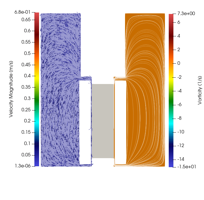
Figure 47: FVM 桶 GIF